Linear Equations

Theorem 2.2.2 also gives a useful way to describe the solutions to a system

$\begin{equation*} A\textbf{x} = \textbf{b} \end{equation*}$

of linear equations. There is a related system

$\begin{equation*} A\textbf{x} = \textbf{0} \end{equation*}$

called the associated homogeneous system, obtained from the original system $A\textbf{x} = \textbf{b}$ by replacing all the constants by zeros. Suppose $\textbf{x}_{1}$ is a solution to $A\textbf{x} = \textbf{b}$ and $\textbf{x}_{0}$ is a solution to $A\textbf{x} = \textbf{0}$ (that is $A\textbf{x}_{1} = \textbf{b}$ and $A\textbf{x}_{0} = \textbf{0}$ ). Then $\textbf{x}_{1} + \textbf{x}_{0}$ is another solution to $A\textbf{x} = \textbf{b}$ . Indeed, Theorem 2.2.2 gives

$\begin{equation*} A(\textbf{x}_{1} + \textbf{x}_{0}) = A\textbf{x}_{1} + A\textbf{x}_{0} = \textbf{b} + \textbf{0} = \textbf{b} \end{equation*}$

This observation has a useful converse.

Theorem :

Suppose $\textbf{x}_{1}$ is any particular solution to the system $A\textbf{x} = \textbf{b}$ of linear equations. Then every solution $\textbf{x}_{2}$ to $A\textbf{x} = \textbf{b}$ has the form

$\begin{equation*} \textbf{x}_{2} = \textbf{x}_{0} + \textbf{x}_{1} \end{equation*}$

for some solution $\textbf{x}_{0}$ of the associated homogeneous system $A\textbf{x} = \textbf{0}$ .

Proof:
Suppose $\textbf{x}_{2}$ is also a solution to $A\textbf{x} = \textbf{b}$ , so that $A\textbf{x}_{2} = \textbf{b}$ . Write $\textbf{x}_{0} = \textbf{x}_{2} - \textbf{x}_{1}$ . Then $\textbf{x}_{2} = \textbf{x}_{0} + \textbf{x}_{1}$ and, using Theorem 2.2.2, we compute

$\begin{equation*} A\textbf{x}_{0} = A(\textbf{x}_{2} - \textbf{x}_{1}) = A\textbf{x}_{2} - A\textbf{x}_{1} = \textbf{b} - \textbf{b} = \textbf{0} \end{equation*}$

Hence $\textbf{x}_{0}$ is a solution to the associated homogeneous system $A\textbf{x} = \textbf{0}$ .

Note that gaussian elimination provides one such representation.

Example :

Express every solution to the following system as the sum of a specific solution plus a solution to the associated homogeneous system.

$\begin{equation*} \arraycolsep=1pt \begin{array}{rrrrrrrrr} x_{1} & - & x_{2} & - & x_{3} & + & 3x_{4} & = & 2 \\ 2x_{1} & - & x_{2} & - & 3x_{3}& + & 4x_{4} & = & 6 \\ x_{1} & & & - & 2x_{3} & + & x_{4} & = & 4 \end{array} \end{equation*}$

Solution:

Gaussian elimination gives $x_{1} = 4 + 2s - t$ , $x_{2} = 2 + s + 2t$ , $x_{3} = s$ , and $x_{4} = t$ where $s$ and $t$ are arbitrary parameters. Hence the general solution can be written

$\begin{equation*} \textbf{x} = \left[ \begin{array}{c} x_{1} \\ x_{2} \\ x_{3} \\ x_{4} \end{array} \right] = \left[ \begin{array}{c} 4 + 2s - t \\ 2 + s + 2t \\ s \\ t \end{array} \right] = \left[ \begin{array}{r} 4 \\ 2 \\ 0 \\ 0 \end{array} \right] + \left( s \left[ \begin{array}{r} 2 \\ 1 \\ 1 \\ 0 \end{array} \right] + t \left[ \begin{array}{r} -1 \\ 2 \\ 0 \\ 1 \end{array} \right] \right) \end{equation*}$

Thus
$\textbf{x}_1 = \left[ \begin{array}{r} 4 \\ 2 \\ 0 \\ 0 \end{array} \right]$
is a particular solution (where $s = 0 = t$ ), and
$\textbf{x}_{0} = s \left[ \begin{array}{r} 2 \\ 1 \\ 1 \\ 0 \end{array} \right] + t \left[ \begin{array}{r} -1 \\ 2 \\ 0 \\ 1 \end{array} \right]$ gives all solutions to the associated homogeneous system. (To see why this is so, carry out the gaussian elimination again but with all the constants set equal to zero.)

The following useful result is included with no proof.

Theorem :

Let $A\textbf{x} = \textbf{b}$ be a system of equations with augmented matrix $\left[ \begin{array}{c|c} A & \textbf{b} \end{array}\right]$ . Write $\text{rank} A = r$ .

1. $\text{rank} \left[ \begin{array}{c|c} A & \textbf{b} \end{array}\right]$ is either $r$ or $r+1$ .

2. The system is consistent if and only if $\text{rank} \left[ \begin{array}{c|c} A & \textbf{b} \end{array}\right] = r$ .

3. The system is inconsistent if and only if $\text{rank} \left[ \begin{array}{c|c} A & \textbf{b} \end{array}\right] = r+1$ .

The Dot Product

Definition 2.5 is not always the easiest way to compute a matrix-vector product $A\textbf{x}$ because it requires that the columns of $A$ be explicitly identified. There is another way to find such a product which uses the matrix $A$ as a whole with no reference to its columns, and hence is useful in practice. The method depends on the following notion.

If $(a_{1}, a_{2}, \dots, a_{n})$ and $(b_{1}, b_{2}, \dots, b_{n})$ are two ordered $n$ -tuples, their $\textbf{dot product}$ is defined to be the number

$\begin{equation*} a_{1}b_{1} + a_{2}b_{2} + \dots + a_{n}b_{n} \end{equation*}$

obtained by multiplying corresponding entries and adding the results.

To see how this relates to matrix products, let $A$ denote a $3 \times 4$ matrix and let $\textbf{x}$ be a $4$ -vector. Writing

$\begin{equation*} \textbf{x} = \left[ \begin{array}{c} x_{1} \\ x_{2} \\ x_{3} \\ x_{4} \end{array} \right] \quad \mbox{ and } \quad A = \left[ \begin{array}{cccc} a_{11} & a_{12} & a_{13} & a_{14} \\ a_{21} & a_{22} & a_{23} & a_{24} \\ a_{31} & a_{32} & a_{33} & a_{34} \end{array} \right] \end{equation*}$

in the notation of Section 2.1, we compute

$\begin{align*} A\textbf{x} = \left[ \begin{array}{cccc} a_{11} & a_{12} & a_{13} & a_{14} \\ a_{21} & a_{22} & a_{23} & a_{24} \\ a_{31} & a_{32} & a_{33} & a_{34} \end{array} \right] \left[ \begin{array}{c} x_{1} \\ x_{2} \\ x_{3} \\ x_{4} \end{array} \right] &= x_{1} \left[ \begin{array}{c} a_{11} \\ a_{21} \\ a_{31} \end{array} \right] + x_{2} \left[ \begin{array}{c} a_{12} \\ a_{22} \\ a_{32} \end{array} \right] + x_{3} \left[ \begin{array}{c} a_{13} \\ a_{23} \\ a_{33} \end{array} \right] + x_{4} \left[ \begin{array}{c} a_{14} \\ a_{24} \\ a_{34} \end{array} \right] \\ &= \left[ \begin{array}{c} a_{11}x_{1} + a_{12}x_{2} + a_{13}x_{3} + a_{14}x_{4} \\ a_{21}x_{1} + a_{22}x_{2} + a_{23}x_{3} + a_{24}x_{4} \\ a_{31}x_{1} + a_{32}x_{2} + a_{33}x_{3} + a_{34}x_{4} \end{array} \right] \end{align*}$

From this we see that each entry of $A\textbf{x}$ is the dot product of the corresponding row of $A$ with $\textbf{x}$ . This computation goes through in general, and we record the result in Theorem 2.2.5.

Theorem 2.2.5 Dot Product Rule

Let $A$ be an $m \times n$ matrix and let $\textbf{x}$ be an $n$ -vector. Then each entry of the vector $A\textbf{x}$ is the dot product of the corresponding row of $A$ with $\textbf{x}$ .

This result is used extensively throughout linear algebra.

If $A$ is $m \times n$ and $\textbf{x}$ is an $n$ -vector, the computation of $A\textbf{x}$ by the dot product rule is simpler than using Definition 2.5 because the computation can be carried out directly with no explicit reference to the columns of $A$ (as in Definition 2.5. The first entry of $A\textbf{x}$ is the dot product of row 1 of $A$ with $\textbf{x}$ . In hand calculations this is computed by going across row one of $A$ , going down the column $\textbf{x}$ , multiplying corresponding entries, and adding the results. The other entries of $A\textbf{x}$ are computed in the same way using the other rows of $A$ with the column $\textbf{x}$ .

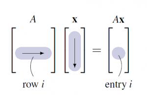
In general, compute entry $i$ of $A\textbf{x}$ as follows (see the diagram):

Go across row $i$ of $A$ and down column $\textbf{x}$ , multiply corresponding entries, and add the results.

As an illustration, we rework Example 2.2.2 using the dot product rule instead of Definition.

Example :

If $A = \left[ \begin{array}{rrrr} 2 & -1 & 3 & 5 \\ 0 & 2 & -3 & 1 \\ -3 & 4 & 1 & 2 \end{array} \right]$
and $\textbf{x} = \left[ \begin{array}{r} 2 \\ 1 \\ 0 \\ -2 \end{array} \right]$ , compute $A\textbf{x}$ .

Solution:
The entries of $A\textbf{x}$ are the dot products of the rows of $A$ with $\textbf{x}$ :

$\begin{equation*} A\textbf{x} = \left[ \begin{array}{rrrr} 2 & -1 & 3 & 5 \\ 0 & 2 & -3 & 1 \\ -3 & 4 & 1 & 2 \end{array} \right] \left[ \begin{array}{r} 2 \\ 1 \\ 0 \\ -2 \end{array} \right] = \left[ \begin{array}{rrrrrrr} 2 \cdot 2 & + & (-1)1 & + & 3 \cdot 0 & + & 5(-2) \\ 0 \cdot 2 & + & 2 \cdot 1 & + & (-3)0 & + & 1(-2) \\ (-3)2 & + & 4 \cdot 1 & + & 1 \cdot 0 & + & 2(-2) \end{array} \right] = \left[ \begin{array}{r} -7 \\ 0 \\ -6 \end{array} \right] \end{equation*}$

Of course, this agrees with the outcome in above Example

Example :

Write the following system of linear equations in the form $A\textbf{x} = \textbf{b}$ .

$\begin{equation*} \arraycolsep=1pt \begin{array}{rrrrrrrrrrr} 5x_{1} & - & x_{2} & + & 2x_{3} & + & x_{4} & - & 3x_{5} & = & 8 \\ x_{1} & + & x_{2} & + & 3x_{3} & - & 5x_{4} & + & 2x_{5} & = & -2 \\ -x_{1} & + & x_{2} & - & 2x_{3} & + & & - & 3x_{5} & = & 0 \end{array} \end{equation*}$

Solution:

Write $A = \left[ \begin{array}{rrrrr} 5 & -1 & 2 & 1 & -3 \\ 1 & 1 & 3 & -5 & 2 \\ -1 & 1 & -2 & 0 & -3 \end{array} \right]$ , $\textbf{b} = \left[ \begin{array}{r} 8 \\ -2 \\ 0 \end{array} \right]$ , and $\textbf{x} = \left[ \begin{array}{c} x_{1} \\ x_{2} \\ x_{3} \\ x_{4} \\ x_{5} \end{array} \right]$ . Then the dot product rule gives $A\textbf{x} = \left[ \arraycolsep=1pt \begin{array}{rrrrrrrrr} 5x_{1} & - & x_{2} & + & 2x_{3} & + & x_{4} & - & 3x_{5} \\ x_{1} & + & x_{2} & + & 3x_{3} & - & 5x_{4} & + & 2x_{5} \\ -x_{1} & + & x_{2} & - & 2x_{3} & & & - & 3x_{5} \end{array} \right]$ , so the entries of $A\textbf{x}$ are the left sides of the equations in the linear system. Hence the system becomes $A\textbf{x} = \textbf{b}$ because matrices are equal if and only corresponding entries are equal.

Example :

If $A$ is the zero $m \times n$ matrix, then $A\textbf{x} = \textbf{0}$ for each $n$ -vector $\textbf{x}$ .

Solution:

For each $k$ , entry $k$ of $A\textbf{x}$ is the dot product of row $k$ of $A$ with $\textbf{x}$ , and this is zero because row $k$ of $A$ consists of zeros.

The Identity Matrix

For each $n > 2$ , the $\textbf{identity matrix}$ $I_{n}$ is the $n \times n$ matrix with 1s on the main diagonal (upper left to lower right), and zeros elsewhere.

The first few identity matrices are

$\begin{equation*} I_{2} = \left[ \begin{array}{rr} 1 & 0 \\ 0 & 1 \end{array} \right], \quad I_{3} = \left[ \begin{array}{rrr} 1 & 0 & 0 \\ 0 & 1 & 0 \\ 0 & 0 & 1 \end{array} \right], \quad I_{4} = \left[ \begin{array}{rrrr} 1 & 0 & 0 & 0 \\ 0 & 1 & 0 & 0 \\ 0 & 0 & 1 & 0 \\ 0 & 0 & 0 & 1 \end{array} \right], \quad \dots \end{equation*}$

In Example 2.2.6 we showed that $I_{3}\textbf{x} = \textbf{x}$ for each $3$ -vector $\textbf{x}$ using Definition 2.5. The following result shows that this holds in general, and is the reason for the name.

Example :

For each $n \geq 2$ we have $I_{n}\textbf{x} = \textbf{x}$ for each $n$ -vector $\textbf{x}$ in $\mathbf{R}^n$ .

Solution:

We verify the case $n = 4$ . Given the $4$ -vector $\textbf{x} = \left[ \begin{array}{c} x_{1} \\ x_{2} \\ x_{3} \\ x_{4} \end{array} \right]$
the dot product rule gives

$\begin{equation*} I_{4}\textbf{x} = \left[\begin{array}{rrrr} 1 & 0 & 0 & 0 \\ 0 & 1 & 0 & 0 \\ 0 & 0 & 1 & 0 \\ 0 & 0 & 0 & 1 \end{array} \right] \left[ \begin{array}{c} x_{1} \\ x_{2} \\ x_{3} \\ x_{4} \end{array} \right] = \left[ \begin{array}{c} x_{1} + 0 + 0 + 0 \\ 0 + x_{2} + 0 + 0 \\ 0 + 0 + x_{3} + 0 \\ 0 + 0 + 0 + x_{4} \end{array} \right] = \left[ \begin{array}{c} x_{1} \\ x_{2} \\ x_{3} \\ x_{4} \end{array} \right] = \vect{x} \end{equation*}$

In general, $I_{n}\textbf{x} = \textbf{x}$ because entry $k$ of $I_{n}\textbf{x}$ is the dot product of row $k$ of $I_{n}$ with $\textbf{x}$ , and row $k$ of $I_{n}$ has $1$ in position $k$ and zeros elsewhere.

Example :

Let $A = \left[ \begin{array}{cccc} \textbf{a}_{1} & \textbf{a}_{2} & \cdots & \textbf{a}_{n} \end{array} \right]$ be any $m \times n$ matrix with columns $\textbf{a}_{1}, \textbf{a}_{2}, \dots, \textbf{a}_{n}$ . If $\textbf{e}_{j}$ denotes column $j$ of the $n \times n$ identity matrix $I_{n}$ , then $A\textbf{e}_{j} = \textbf{a}_{j}$ for each $j = 1, 2, \dots, n$ .

Solution:

Write $\textbf{e}_{j} = \left[ \begin{array}{c} t_{1} \\ t_{2} \\ \vdots \\ t_{n} \end{array} \right]$
where $t_{j} = 1$ , but $t_{i} = 0$ for all $i \neq j$ . Then Theorem 2.2.5 gives

$\begin{equation*} A\textbf{e}_{j} = t_{1}\textbf{a}_{1} + \dots + t_{j}\textbf{a}_{j} + \dots + t_{n}\textbf{a}_{n} = 0 + \dots + \textbf{a}_{j} + \dots + 0 = \textbf{a}_{j} \end{equation*}$

Example 2.2.12will be referred to later; for now we use it to prove:

Theorem :

Let $A$ and $B$ be $m \times n$ matrices. If $A\textbf{x} = B\textbf{x}$ for all $\textbf{x}$ in $\mathbf{R}^n$ , then $A = B$ .

Proof:

Write $A = \left[ \begin{array}{cccc} \textbf{a}_{1} & \textbf{a}_{2} & \cdots & \textbf{a}_{n} \end{array} \right]$ and $B = \left[ \begin{array}{cccc} \textbf{b}_{1} & \textbf{b}_{2} & \cdots & \textbf{b}_{n} \end{array} \right]$ and in terms of their columns. It is enough to show that $\textbf{a}_{k} = \textbf{b}_{k}$ holds for all $k$ . But we are assuming that $A\textbf{e}_{k} = B\textbf{e}_{k}$ , which gives $\textbf{a}_{k} = \textbf{b}_{k}$ by Example 2.2.12.

We have introduced matrix-vector multiplication as a new way to think about systems of linear equations. But it has several other uses as well. It turns out that many geometric operations can be described using matrix multiplication, and we now investigate how this happens. As a bonus, this description provides a geometric “picture” of a matrix by revealing the effect on a vector when it is multiplied by $A$ . This “geometric view” of matrices is a fundamental tool in understanding them.

Matrix Multiplication

In Section 2.2 matrix-vector products were introduced. If $A$ is an $m \times n$ matrix, the product $A\textbf{x}$ was defined for any $n$ -column $\vect{x}$ in $\mathbf{R}^n$ as follows: If $A = \left[ \begin{array}{cccc} \textbf{a}_{1} & \textbf{a}_{2} & \cdots & \textbf{a}_{n} \end{array} \right]$ where the $\textbf{a}_{j}$ are the columns of $A$ , and if $\textbf{x} = \left[ \begin{array}{c} x_{1} \\ x_{2} \\ \vdots \\ x_{n} \end{array} \right]$ ,

Definition 2.5 reads

(2.5) $\begin{equation*} A\textbf{x} = x_{1}\textbf{a}_{1} + x_{2}\textbf{a}_{2} + \cdots + x_{n}\textbf{a}_{n} \end{equation*}$

This was motivated as a way of describing systems of linear equations with coefficient matrix $A$ . Indeed every such system has the form $A\textbf{x} = \textbf{b}$ where $\textbf{b}$ is the column of constants.

In this section we extend this matrix-vector multiplication to a way of multiplying matrices in general, and then investigate matrix algebra for its own sake. While it shares several properties of ordinary arithmetic, it will soon become clear that matrix arithmetic is different in a number of ways.

Matrix Multiplication

Let $A$ be an $m \times n$ matrix, let $B$ be an $n \times k$ matrix, and write $B = \left[ \begin{array}{cccc} \textbf{b}_{1} & \textbf{b}_{2} & \cdots & \textbf{b}_{k} \end{array} \right]$ where $\textbf{b}_{j}$ is column $j$ of $B$ for each $j$ . The product matrix $AB$ is the $m \times k$ matrix defined as follows:

$\begin{equation*} AB = A \left[ \begin{array}{cccc} \textbf{b}_{1} & \textbf{b}_{2} & \cdots & \textbf{b}_{k} \end{array} \right] = \left[ \begin{array}{cccc} A\textbf{b}_{1} & A\textbf{b}_{2} & \cdots & A\textbf{b}_{k} \end{array} \right] \end{equation*}$

Thus the product matrix $AB$ is given in terms of its columns $A\textbf{b}_{1}, A\textbf{b}_{2}, \dots, A\textbf{b}_{n}$ : Column $j$ of $AB$ is the matrix-vector product $A\textbf{b}_{j}$ of $A$ and the corresponding column $\textbf{b}_{j}$ of $B$ . Note that each such product $A\textbf{b}_{j}$ makes sense by Definition 2.5 because $A$ is $m \times n$ and each $\vect{b}_{j}$ is in $\mathbf{R}^n$ (since $B$ has $n$ rows). Note also that if $B$ is a column matrix, this definition reduces to Definition 2.5 for matrix-vector multiplication.

Given matrices $A$ and $B$ , Definition 2.9 and the above computation give

$\begin{equation*} A(B\vec{x}) = \left[ \begin{array}{cccc} A\vec{b}_{1} & A\vec{b}_{2} & \cdots & A\vec{b}_{n} \end{array} \right] \vec{x} = (AB)\vec{x} \end{equation*}$

for all $\vec{x}$ in $\mathbf{R}^k$ . We record this for reference.

Theorem :

Let $A$ be an $m \times n$ matrix and let $B$ be an $n \times k$ matrix. Then the product matrix $AB$ is $m \times k$ and satisfies

$\begin{equation*} A(B\vec{x}) = (AB)\vec{x} \quad \mbox{ for all } \vec{x} \mbox{ in } \mathbf{R}^{k} \end{equation*}$

Here is an example of how to compute the product $AB$ of two matrices using Definition 2.9.

Example :

Compute $AB$ if $A = \left[ \begin{array}{rrr} 2 & 3 & 5 \\ 1 & 4 & 7 \\ 0 & 1 & 8 \end{array} \right]$
and
$B = \left[\begin{array}{rr} 8 & 9 \\ 7 & 2 \\ 6 & 1 \end{array} \right]$ .

Solution:

The columns of $B$ are
$\vec{b}_{1} = \left[ \begin{array}{r} 8 \\ 7 \\ 6 \end{array} \right]$ and $\vec{b}_{2} = \left[ \begin{array}{r} 9 \\ 2 \\ 1 \end{array} \right]$ , so Definition 2.5 gives

$\begin{equation*} A\vec{b}_{1} = \left[ \begin{array}{rrr} 2 & 3 & 5 \\ 1 & 4 & 7 \\ 0 & 1 & 8 \end{array} \right] \left[ \begin{array}{r} 8 \\ 7 \\ 6 \end{array} \right] = \left[ \begin{array}{r} 67 \\ 78 \\ 55 \end{array} \right] \mbox{ and } A\vec{b}_{2} = \left[ \begin{array}{rrr} 2 & 3 & 5 \\ 1 & 4 & 7 \\ 0 & 1 & 8 \end{array} \right] \left[ \begin{array}{r} 9 \\ 2 \\ 1 \end{array} \right] = \left[\begin{array}{r} 29 \\ 24 \\ 10 \end{array} \right] \end{equation*}$

Hence Definition 2.9 above gives $AB = \left[ \begin{array}{cc} A\vec{b}_{1} & A\vec{b}_{2} \end{array} \right] = \left[ \begin{array}{rr} 67 & 29 \\ 78 & 24 \\ 55 & 10 \end{array} \right]$ .

While Definition 2.9 is important, there is another way to compute the matrix product $AB$ that gives a way to calculate each individual entry. In Section 2.2 we defined the dot product of two $n$ -tuples to be the sum of the products of corresponding entries. We went on to show (Theorem 2.2.5) that if $A$ is an $m \times n$ matrix and $\vec{x}$ is an $n$ -vector, then entry $j$ of the product $A\vec{x}$ is the dot product of row $j$ of $A$ with $\vec{x}$ . This observation was called the “dot product rule” for matrix-vector multiplication, and the next theorem shows that it extends to matrix multiplication in general.

Dot Product Rule

Let $A$ and $B$ be matrices of sizes $m \times n$ and $n \times k$ , respectively. Then the $(i, j)$ -entry of $AB$ is the dot
product of row $i$ of $A$ with column $j$ of $B$ .

Proof:

Write $B = \left[ \begin{array}{cccc} \vec{b}_{1} & \vec{b}_{2} & \cdots & \vec{b}_{n} \end{array} \right]$ in terms of its columns. Then $A\vec{b}_{j}$ is column $j$ of $AB$ for each $j$ . Hence the $(i, j)$ -entry of $AB$ is entry $i$ of $A\vec{b}_{j}$ , which is the dot product of row $i$ of $A$ with $\vec{b}_{j}$ . This proves the theorem.

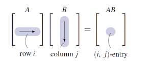
Thus to compute the $(i, j)$ -entry of $AB$ , proceed as follows (see the diagram):

Go across row $i$ of $A$ , and down column $j$ of $B$ , multiply corresponding entries, and add the results.

Note that this requires that the rows of $A$ must be the same length as the columns of $B$ . The following rule is useful for remembering this and for deciding the size of the product matrix $AB$ .

Compatibility Rule

Let $A$ and $B$ denote matrices. If $A$ is $m \times n$ and $B$ is $n^\prime \times k$ , the product $AB$ can be formed if and only if $n=n^\prime$ . In this case the size of the product matrix $AB$ is $m \times k$ , and we say that $AB$ is defined, or that $A$ and $B$ are compatible for multiplication.

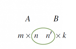
The diagram provides a useful mnemonic for remembering this. We adopt the following convention:

Whenever a product of matrices is written, it is tacitly assumed that the sizes of the factors are such that the product is defined.

To illustrate the dot product rule, we recompute the matrix product in Example .

Example :

Compute $AB$ if $A = \left[ \begin{array}{rrr} 2 & 3 & 5 \\ 1 & 4 & 7 \\ 0 & 1 & 8 \end{array} \right]$
and $B = \left[ \begin{array}{rr} 8 & 9 \\ 7 & 2 \\ 6 & 1 \end{array} \right]$ .

Solution:

Here $A$ is $3 \times 3$ and $B$ is $3 \times 2$ , so the product matrix $AB$ is defined and will be of size $3 \times 2$ . Theorem 2.3.2 gives each entry of $AB$ as the dot product of the corresponding row of $A$ with the corresponding column of $B_{j}$ that is,

$\begin{equation*} AB = \left[ \begin{array}{rrr} 2 & 3 & 5 \\ 1 & 4 & 7 \\ 0 & 1 & 8 \end{array} \right] \left[ \begin{array}{rr} 8 & 9 \\ 7 & 2 \\ 6 & 1 \end{array} \right]= \left[ \arraycolsep=8pt \begin{array}{cc} 2 \cdot 8 + 3 \cdot 7 + 5 \cdot 6 & 2 \cdot 9 + 3 \cdot 2 + 5 \cdot 1 \\ 1 \cdot 8 + 4 \cdot 7 + 7 \cdot 6 & 1 \cdot 9 + 4 \cdot 2 + 7 \cdot 1 \\ 0 \cdot 8 + 1 \cdot 7 + 8 \cdot 6 & 0 \cdot 9 + 1 \cdot 2 + 8 \cdot 1 \end{array} \right] = \left[ \begin{array}{rr} 67 & 29 \\ 78 & 24 \\ 55 & 10 \end{array} \right] \end{equation*}$

Of course, this agrees with Example

Example :

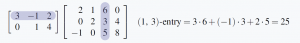
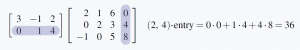
Compute the $(1, 3)$ – and $(2, 4)$ -entries of $AB$ where

$\begin{equation*} A = \left[ \begin{array}{rrr} 3 & -1 & 2 \\ 0 & 1 & 4 \end{array} \right] \mbox{ and } B = \left[ \begin{array}{rrrr} 2 & 1 & 6 & 0 \\ 0 & 2 & 3 & 4 \\ -1 & 0 & 5 & 8 \end{array} \right]. \end{equation*}$

Then compute $AB$ .

Solution:

The $(1, 3)$ -entry of $AB$ is the dot product of row 1 of $A$ and column 3 of $B$ (highlighted in the following display), computed by multiplying corresponding entries and adding the results.

Similarly, the $(2, 4)$ -entry of $AB$ involves row 2 of $A$ and column 4 of $B$ .

Since $A$ is $2 \times 3$ and $B$ is $3 \times 4$ , the product is $2 \times 4$ .

$\begin{equation*} AB = \left[ \begin{array}{rrr} 3 & -1 & 2 \\ 0 & 1 & 4 \end{array} \right] \left[ \begin{array}{rrrr} 2 & 1 & 6 & 0 \\ 0 & 2 & 3 & 4 \\ -1 & 0 & 5 & 8 \end{array} \right] = \left[ \begin{array}{rrrr} 4 & 1 & 25 & 12 \\ -4 & 2 & 23 & 36 \end{array} \right] \end{equation*}$

Example :

If $A = \left[ \begin{array}{ccc} 1 & 3 & 2\end{array}\right]$ and $B = \left[ \begin{array}{r} 5 \\ 6 \\ 4 \end{array} \right]$ , compute $A^{2}$ , $AB$ , $BA$ , and $B^{2}$ when they are defined.

Solution:

Here, $A$ is a $1 \times 3$ matrix and $B$ is a $3 \times 1$ matrix, so $A^{2}$ and $B^{2}$ are not defined. However, the compatibility rule reads

$\begin{equation*} \begin{array}{ccc} \begin{array}{cc} A & B\\ 1 \times 3 & 3 \times 1 \end{array} & \mbox{ and } & \begin{array}{cc} B & A \\ 3 \times 1 & 1 \times 3 \end{array} \end{array} \end{equation*}$

so both $AB$ and $BA$ can be formed and these are $1 \times 1$ and $3 \times 3$ matrices, respectively.

$\begin{equation*} AB = \left[ \begin{array}{rrr} 1 & 3 & 2 \end{array} \right] \left[ \begin{array}{r} 5 \\ 6 \\ 4 \end{array} \right] = \left[ \begin{array}{c} 1 \cdot 5 + 3 \cdot 6 + 2 \cdot 4 \end{array} \right] = \arraycolsep=1.5pt \left[ \begin{array}{c} 31 \end{array}\right] \end{equation*}$

$\begin{equation*} BA = \left[ \begin{array}{r} 5 \\ 6 \\ 4 \end{array} \right] \left[ \begin{array}{rrr} 1 & 3 & 2 \end{array} \right] = \left[ \begin{array}{rrr} 5 \cdot 1 & 5 \cdot 3 & 5 \cdot 2 \\ 6 \cdot 1 & 6 \cdot 3 & 6 \cdot 2 \\ 4 \cdot 1 & 4 \cdot 3 & 4 \cdot 2 \end{array} \right] = \left[ \begin{array}{rrr} 5 & 15 & 10 \\ 6 & 18 & 12 \\ 4 & 12 & 8 \end{array} \right \end{equation*}$

Unlike numerical multiplication, matrix products $AB$ and $BA$ need not be equal. In fact they need not even be the same size, as Example 2.3.5 shows. It turns out to be rare that $AB = BA$ (although it is by no means impossible), and $A$ and $B$ are said to commute when this happens.

Example :

Let $A = \left[ \begin{array}{rr} 6 & 9 \\ -4 & -6 \end{array} \right]$ and $B = \left[ \begin{array}{rr} 1 & 2 \\ -1 & 0 \end{array} \right]$ . Compute $A^{2}$ , $AB$ , $BA$ .

Solution:
$A^{2} = \left[ \begin{array}{rr} 6 & 9 \\ -4 & -6 \end{array} \right] \left[ \begin{array}{rr} 6 & 9 \\ -4 & -6 \end{array} \right] = \left[ \begin{array}{rr} 0 & 0 \\ 0 & 0 \end{array} \right]$ , so $A^{2} = 0$ can occur even if $A \neq 0$ . Next,

$\begin{align*} AB & = \left[ \begin{array}{rr} 6 & 9 \\ -4 & -6 \end{array} \right] \left[ \begin{array}{rr} 1 & 2 \\ -1 & 0 \end{array} \right] = \left[ \begin{array}{rr} -3 & 12 \\ 2 & -8 \end{array} \right] \\ BA & = \left[ \begin{array}{rr} 1 & 2 \\ -1 & 0 \end{array} \right] \left[ \begin{array}{rr} 6 & 9 \\ -4 & -6 \end{array} \right] = \left[ \begin{array}{rr} -2 & -3 \\ -6 & -9 \end{array} \right] \end{align*}$

Hence $AB \neq BA$ , even though $AB$ and $BA$ are the same size.

Example :

If $A$ is any matrix, then $IA = A$ and $AI = A$ , and where $I$ denotes an identity matrix of a size so that the multiplications are defined.

Solution:

These both follow from the dot product rule as the reader should verify. For a more formal proof, write $A = \left[ \begin{array}{rrrr} \vec{a}_{1} & \vec{a}_{2} & \cdots & \vec{a}_{n} \end{array} \right]$ where $\vec{a}_{j}$ is column $j$ of $A$ . Then Definition 2.9 and Example 2.2.1 give

$\begin{equation*} IA = \left[ \begin{array}{rrrr} I\vec{a}_{1} & I\vec{a}_{2} & \cdots & I\vec{a}_{n} \end{array} \right] = \left[ \begin{array}{rrrr} \vect{a}_{1} & \vect{a}_{2} & \cdots & \vect{a}_{n} \end{array} \right] = A \end{equation*}$

If $\vec{e}_{j}$ denotes column $j$ of $I$ , then $A\vec{e}_{j} = \vec{a}_{j}$ for each $j$ by Example 2.2.12. Hence Definition 2.9 gives:

$\begin{equation*} AI = A \left[ \begin{array}{rrrr} \vec{e}_{1} & \vec{e}_{2} & \cdots & \vec{e}_{n} \end{array} \right] = \left[ \begin{array}{rrrr} A\vec{e}_{1} & A\vec{e}_{2} & \cdots & A\vec{e}_{n} \end{array} \right] = \left[ \begin{array}{rrrr} \vec{a}_{1} & \vec{a}_{2} & \cdots & \vec{a}_{n} \end{array} \right] = A \end{equation*}$

The following theorem collects several results about matrix multiplication that are used everywhere in linear algebra.

Theorem :

Assume that $a$ is any scalar, and that $A$ , $B$ , and $C$ are matrices of sizes such that the indicated matrix products are defined. Then:

1. $IA = A$ and $AI = A$ where $I$ denotes an identity matrix.

2. $A(BC) = (AB)C$ .

3. $A(B + C) = AB + AC$ .

4. $(B + C)A = BA + CA$ .

5. $a(AB) = (aA)B = A(aB)$ .

6. $(AB)^{T} = B^{T}A^{T}$ .

Proof:

Condition (1) is Example 2.3.7; we prove (2), (4), and (6) and leave (3) and (5) as exercises.
1. If $C = \left[ \begin{array}{cccc} \vec{c}_{1} & \vec{c}_{2} & \cdots & \vec{c}_{k} \end{array} \right]$ in terms of its columns, then $BC = \left[ \begin{array}{cccc} B\vec{c}_{1} & B\vec{c}_{2} & \cdots & B\vec{c}_{k} \end{array} \right]$ by Definition 2.9, so

$\begin{equation*} \begin{array}{lllll} A(BC) & = & \left[ \begin{array}{rrrr} A(B\vec{c}_{1}) & A(B\vec{c}_{2}) & \cdots & A(B\vec{c}_{k}) \end{array} \right] & & \mbox{Definition 2.9} \\ & & & & \\ & = & \left[ \begin{array}{rrrr} (AB)\vec{c}_{1} & (AB)\vec{c}_{2} & \cdots & (AB)\vec{c}_{k}) \end{array} \right] & & \mbox{Theorem 2.3.1} \\ & & & & \\ & = & (AB)C & & \mbox{Definition 2.9} \end{array} \end{equation*}$

4. We know (Theorem 2.2.) that $(B + C)\vec{x} = B\vec{x} + C\vec{x}$ holds for every column $\vec{x}$ . If we write $A = \left[ \begin{array}{rrrr} \vec{a}_{1} & \vec{a}_{2} & \cdots & \vec{a}_{n} \end{array} \right]$ in terms of its columns, we get

$\begin{equation*} \begin{array}{lllll} (B + C)A & = & \left[ \begin{array}{rrrr} (B + C)\vec{a}_{1} & (B + C)\vec{a}_{2} & \cdots & (B + C)\vec{a}_{n} \end{array} \right] & & \mbox{Definition 2.9} \\ & & & & \\ & = & \left[ \begin{array}{rrrr} B\vec{a}_{1} + C\vec{a}_{1} & B\vec{a}_{2} + C\vec{a}_{2} & \cdots & B\vec{a}_{n} + C\vec{a}_{n} \end{array} \right] & & \mbox{Theorem 2.2.2} \\ & & & & \\ & = & \left[ \begin{array}{rrrr} B\vec{a}_{1} & B\vec{a}_{2} & \cdots & B\vec{a}_{n} \end{array} \right] + \left[ \begin{array}{rrrr} C\vec{a}_{1} & C\vec{a}_{2} & \cdots & C\vec{a}_{n} \end{array} \right] & & \mbox{Adding Columns} \\ & & & & \\ & = & BA + CA & & \mbox{Definition 2.9} \end{array} \end{equation*}$

6. As in Section 2.1, write $A = [a_{ij}]$ and $B = [b_{ij}]$ , so that $A^{T} = [a^\prime_{ij}]$ and $B^{T} = [b^\prime_{ij}]$ where $a^\prime_{ij} = a_{ji}$ and $b^\prime_{ji} = b_{ij}$ for all $i$ and $j$ . If $c_{ij}$ denotes the $(i, j)$ -entry of $B^{T}A^{T}$ , then $c_{ij}$ is the dot product of row $i$ of $B^{T}$ with column $j$ of $A^{T}$ . Hence

$\begin{align*} c_{ij} = b_{i1}^\prime a_{1j}^\prime + b_{i2}^\prime a_{2j}^\prime + \cdots + b_{im}^\prime a_{mj}^\prime &= b_{1i} a_{j1} + b_{2i} a_{j2} + \cdots + b_{mi} a_{jm} \\ &= a_{j1}b_{1i} + a_{j2}b_{2i} + \cdots + a_{jm}b_{mi} \end{align*}$

But this is the dot product of row $j$ of $A$ with column $i$ of $B$ ; that is, the $(j, i)$ -entry of $AB$ ; that is, the $(i, j)$ -entry of $(AB)^{T}$ . This proves (6).

Property 2 in Theorem 2.3.3 is called the associative law of matrix multiplication. It asserts that the equation $A(BC) = (AB)C$ holds for all matrices (if the products are defined). Hence this product is the same no matter how it is formed, and so is written simply as $ABC$ . This extends: The product $ABCD$ of four matrices can be formed several ways—for example, $(AB)(CD)$ , $[A(BC)]D$ , and $A[B(CD)]$ —but the associative law implies that they are all equal and so are written as $ABCD$ . A similar remark applies in general: Matrix products can be written unambiguously with no parentheses.

However, a note of caution about matrix multiplication must be taken: The fact that $AB$ and $BA$ need not be equal means that the order of the factors is important in a product of matrices. For example $ABCD$ and $ADCB$ may not be equal.

Warning:
If the order of the factors in a product of matrices is changed, the product matrix may change (or may not be defined). Ignoring this warning is a source of many errors by students of linear algebra!}

Properties 3 and 4 in Theorem 2.3.3 are called distributive laws. They assert that $A(B + C) = AB + AC$ and $(B + C)A = BA + CA$ hold whenever the sums and products are defined. These rules extend to more than two terms and, together with Property 5, ensure that many manipulations familiar from ordinary algebra extend to matrices. For example

$\begin{align*} A(2B - 3C + D - 5E) & = 2AB - 3AC + AD - 5AE \\ (A + 3C - 2D)B & = AB + 3CB - 2DB \end{align*}$

Note again that the warning is in effect: For example $A(B - C)$ need not equal $AB - CA$ . These rules make possible a lot of simplification of matrix expressions.

Simplify the expression $A(BC - CD) + A(C - B)D - AB(C - D)$ .

Solution:

$\begin{align*} A(BC - CD) + A(C - B)D - AB(C - D) &= A(BC) - A(CD) + (AC-AB)D - (AB)C + (AB)D \\ &= ABC - ACD + ACD - ABD - ABC + ABD \\ &= 0 \end{align*}$

Matrix Inverse

Three basic operations on matrices, addition, multiplication, and subtraction, are analogs for matrices of the same operations for numbers. In this section we introduce the matrix analog of numerical division.

To begin, consider how a numerical equation $ax = b$ is solved when $a$ and $b$ are known numbers. If $a = 0$ , there is no solution (unless $b = 0$ ). But if $a \neq 0$ , we can multiply both sides by the inverse $a^{-1} = \frac{1}{a}$ to obtain the solution $x = a^{-1}b$ . Of course multiplying by $a^{-1}$ is just dividing by $a$ , and the property of $a^{-1}$ that makes this work is that $a^{-1}a = 1$ . Moreover, we saw in Section~?? that the role that $1$ plays in arithmetic is played in matrix algebra by the identity matrix $I$ . This suggests the following definition.

If $A$ is a square matrix, a matrix $B$ is called an inverse of $A$ if and only if

$\begin{equation*} AB = I \quad \mbox{ and } \quad BA = I \end{equation*}$

A matrix $A$ that has an inverse is called an $\textbf{invertible matrix}.$

Note that only square matrices have inverses. Even though it is plausible that nonsquare matrices $A$ and $B$ could exist such that $AB = I_{m}$ and $BA = I_{n}$ , where $A$ is $m \times n$ and $B$ is $n \times m$ , we claim that this forces $n = m$ . Indeed, if $m < n$ there exists a nonzero column $\vec{x}$ such that $A\vec{x} = \vec{0}$ (by Theorem 1.3.1), so $\vec{x} = I_{n}\vec{x} = (BA)\vec{x} = B(A\vec{x}) = B(\vec{0}) = \vec{0}$ , a contradiction. Hence $m \geq n$ . Similarly, the condition $AB = I_{m}$ implies that $n \geq m$ . Hence $m = n$ so $A$ is square.}

Example :

Show that $B = \left[ \begin{array}{rr} -1 & 1 \\ 1 & 0 \end{array} \right]$
is an inverse of $A = \left[ \begin{array}{rr} 0 & 1 \\ 1 & 1 \end{array} \right]$ .

Solution:

Compute $AB$ and $BA$ .

$\begin{equation*} AB = \left[ \begin{array}{rr} 0 & 1 \\ 1 & 1 \end{array} \right] \left[ \begin{array}{rr} -1 & 1 \\ 1 & 0 \end{array} \right] = \left[ \begin{array}{rr} 1 & 0 \\ 0 & 1 \end{array} \right] \quad BA = \left[ \begin{array}{rr} -1 & 1 \\ 1 & 0 \end{array} \right] \left[ \begin{array}{rr} 0 & 1 \\ 1 & 1 \end{array} \right] = \left[ \begin{array}{rr} 1 & 0 \\ 0 & 1 \end{array} \right] \end{equation*}$

Hence $AB = I = BA$ , so $B$ is indeed an inverse of $A$ .

Show that $A = \left[ \begin{array}{rr} 0 & 0 \\ 1 & 3 \end{array} \right]$
has no inverse.

Solution:
Let $B = \left[ \begin{array}{rr} a & b \\ c & d \end{array} \right]$
denote an arbitrary $2 \times 2$ matrix. Then

$\begin{equation*} AB = \left[ \begin{array}{rr} 0 & 0 \\ 1 & 3 \end{array} \right] \left[ \begin{array}{rr} a & b \\ c & d \end{array} \right] = \left[ \begin{array}{cc} 0 & 0 \\ a + 3c & b + 3d \end{array} \right] \end{equation*}$

so $AB$ has a row of zeros. Hence $AB$ cannot equal $I$ for any $B$ .

The argument in Example 2.4.2 shows that no zero matrix has an inverse. But Example 2.4.2 also shows that, unlike arithmetic, it is possible for a nonzero matrix to have no inverse. However, if a matrix does have an inverse, it has only one.

Theorem :

If $B$ and $C$ are both inverses of $A$ , then $B = C$ .

Proof:

Since $B$ and $C$ are both inverses of $A$ , we have $CA = I = AB$ . Hence

$\begin{equation*} B = IB = (CA)B = C(AB) = CI = C \end{equation*}$

If $A$ is an invertible matrix, the (unique) inverse of $A$ is denoted $A^{-1}$ . Hence $A^{-1}$ (when it exists) is a square matrix of the same size as $A$ with the property that

$\begin{equation*} AA^{-1} = I \quad \mbox{ and } \quad A^{-1}A = I \end{equation*}$

These equations characterize $A^{-1}$ in the following sense:

Inverse Criterion: If somehow a matrix $B$ can be found such that $AB = I$ and $BA = I$ , then $A$ is invertible and $B$ is the inverse of $A$ ; in symbols, $B = A^{-1}$ .}

This is a way to verify that the inverse of a matrix exists. Example 2.3.3 and Example 2.3.4 offer illustrations.

Example 2.4.3

If $A = \left[ \begin{array}{rr} 0 & -1 \\ 1 & -1 \end{array} \right]$ , show that $A^{3} = I$ and so find $A^{-1}$ .

Solution:

We have $A^{2} = \left[ \begin{array}{rr} 0 & -1 \\ 1 & -1 \end{array} \right] \left[ \begin{array}{rr} 0 & -1 \\ 1 & -1 \end{array} \right] = \left[ \begin{array}{rr} -1 & 1 \\ -1 & 0 \end{array} \right]$ , and so

$\begin{equation*} A^{3} = A^{2}A = \left[ \begin{array}{rr} -1 & 1 \\ -1 & 0 \end{array} \right] \left[ \begin{array}{rr} 0 & -1 \\ 1 & -1 \end{array} \right] = \left[ \begin{array}{rr} 1 & 0 \\ 0 & 1 \end{array} \right] = I \end{equation*}$

Hence $A^{3} = I$ , as asserted. This can be written as $A^{2}A = I = AA^{2}$ , so it shows that $A^{2}$ is the inverse of $A$ . That is, $A^{-1} = A^{2} = \left[ \begin{array}{rr} -1 & 1 \\ -1 & 0 \end{array} \right]$ .

The next example presents a useful formula for the inverse of a $2 \times 2$ matrix $A = \left[ \begin{array}{cc} a & b \\ c & d \end{array} \right]$ when it exists. To state it, we define the $\textbf{determinant}$ $\func{det }A$ and the $\textbf{adjugate}$ $\func{adj }A$ of the matrix $A$ as follows:

$\begin{equation*} \func{det}\left[ \begin{array}{cc} a & b \\ c & d \end{array} \right] = ad - bc, \quad \mbox{ and } \quad \func{adj} \left[ \begin{array}{cc} a & b \\ c & d \end{array} \right] = \left[ \begin{array}{rr} d & -b \\ -c & a \end{array} \right] \end{equation*}$

If $A = \left[ \begin{array}{cc} a & b \\ c & d \end{array} \right]$ , show that $A$ has an inverse if and only if $\func{det } A \neq 0$ , and in this case

$\begin{equation*} A^{-1} = \frac{1}{\func{det } A} \func{adj } A \end{equation*}$

Solution:
For convenience, write $e = \func{det } A = ad - bc$ and
$B = \func{adj } A = \left[ \begin{array}{rr} d & -b \\ -c & a \end{array} \right]$ . Then $AB = eI = BA$ as the reader can verify. So if $e \neq 0$ , scalar multiplication by $\frac{1}{e}$ gives

$\begin{equation*} A(\frac{1}{e}B) = I = (\frac{1}{e}B)A \end{equation*}$

Hence $A$ is invertible and $A^{-1} = \frac{1}{e}B$ . Thus it remains only to show that if $A^{-1}$ exists, then $e \neq 0$ .

We prove this by showing that assuming $e = 0$ leads to a contradiction. In fact, if $e = 0$ , then $AB = eI = 0$ , so left multiplication by $A^{-1}$ gives $A^{-1}AB = A^{-1}0$ ; that is, $IB = 0$ , so $B = 0$ . But this implies that $a$ , $b$ , $c$ , and $d$ are all zero, so $A = 0$ , contrary to the assumption that $A^{-1}$ exists.

As an illustration, if $A = \left[ \begin{array}{rr} 2 & 4 \\ -3 & 8 \end{array} \right]$
then $\func{det } A = 2 \cdot 8 - 4 \cdot (-3) = 28 \neq 0$ . Hence $A$ is invertible and $A^{-1} = \frac{1}{\func{det } A} \func{adj } A = \frac{1}{28} \left[ \begin{array}{rr} 8 &-4 \\ 3 & 2 \end{array} \right]$ , as the reader is invited to verify.

Inverse and Linear systems

Matrix inverses can be used to solve certain systems of linear equations. Recall that a $\textit{system}$ of linear equations can be written as a $\textit{single}$ matrix equation

$\begin{equation*} A\vec{x} = \vec{b} \end{equation*}$

where $A$ and $\vec{b}$ are known and $\vec{x}$ is to be determined. If $A$ is invertible, we multiply each side of the equation on the left by $A^{-1}$ to get

$\begin{align*} A^{-1}A\vec{x} &= A^{-1}\vec{b} \\ I\vec{x} &= A^{-1}\vec{b} \\ \vec{x} &= A^{-1}\vec{b} \end{align*}$

This gives the solution to the system of equations (the reader should verify that $\vec{x} = A^{-1}\vec{b}$ really does satisfy $A\vec{x} = \vec{b}$ ). Furthermore, the argument shows that if $\vec{x}$ is $\textit{any}$ solution, then necessarily $\vec{x} = A^{-1}\vec{b}$ , so the solution is unique. Of course the technique works only when the coefficient matrix $A$ has an inverse. This proves Theorem 2.4.2.

Theorem 2.4.2

Suppose a system of $n$ equations in $n$ variables is written in matrix form as

$\begin{equation*} A\vec{x} = \vec{b} \end{equation*}$

If the $n \times n$ coefficient matrix $A$ is invertible, the system has the unique solution

$\begin{equation*} \vec{x} = A^{-1}\vec{b} \end{equation*}$

Use Example 2.4.4 to solve the system $\left\lbrace \arraycolsep=1pt \begin{array}{rrrrr} 5x_{1} & - & 3x_{2} & = & -4 \\ 7x_{1} & + & 4x_{2} & = & 8 \end{array} \right.$ .

Solution:

In matrix form this is $A\vec{x} = \vec{b}$ where $A = \left[ \begin{array}{rr} 5 & -3 \\ 7 & 4 \end{array} \right]$ , $\vec{x} = \left[ \begin{array}{c} x_{1} \\ x_{2} \end{array} \right]$ , and $\vec{b} = \left[ \begin{array}{r} -4 \\ 8 \end{array} \right]$ . Then $\func{det } A = 5 \cdot 4 - (-3) \cdot 7 = 41$ , so $A$ is invertible and $A^{-1} = \frac{1}{41} \left[ \begin{array}{rr} 4 & 3 \\ -7 & 5 \end{array} \right]$
by Example 2.4.4. Thus Theorem 2.4.2 gives

$\begin{equation*} \vec{x} = A^{-1}\vec{b} = \frac{1}{41} \left[ \begin{array}{rr} 4 & 3 \\ -7 & 5 \end{array} \right] \left[ \begin{array}{r} -4 \\ 8 \end{array} \right] = \frac{1}{41} \left[ \begin{array}{r} 8 \\ 68 \end{array} \right] \end{equation*}$

so the solution is $x_{1} = \frac{8}{41}$ and $x_{2} = \frac{68}{41}$ .

An inversion method

If a matrix $A$ is $n \times n$ and invertible, it is desirable to have an efficient technique for finding the inverse.

Matrix Inversion Algorithm

If $A$ is an invertible (square) matrix, there exists a sequence of elementary row operations that carry $A$ to the identity matrix $I$ of the same size, written $A \to I$ . This same series of row operations carries $I$ to $A^{-1}$ ; that is, $I \to A^{-1}$ . The algorithm can be summarized as follows:

$\begin{equation*} \left[ \begin{array}{cc} A & I \end{array} \right] \rightarrow \left[ \begin{array}{cc} I & A^{-1} \end{array} \right] \end{equation*}$

where the row operations on $A$ and $I$ are carried out simultaneously.

Use the inversion algorithm to find the inverse of the matrix

$\begin{equation*} A = \left[ \begin{array}{rrr} 2 & 7 & 1 \\ 1 & 4 & -1 \\ 1 & 3 & 0 \end{array} \right] \end{equation*}$

Solution:

Apply elementary row operations to the double matrix

$\begin{equation*} \left[ \begin{array}{rrr} A & I \end{array} \right] = \left[ \begin{array}{rrr|rrr} 2 & 7 & 1 & 1 & 0 & 0 \\ 1 & 4 & -1 & 0 & 1 & 0 \\ 1 & 3 & 0 & 0 & 0 & 1 \end{array} \right] \end{equation*}$

so as to carry $A$ to $I$ . First interchange rows 1 and 2.

$\begin{equation*} \left[ \begin{array}{rrr|rrr} 1 & 4 & -1 & 0 & 1 & 0 \\ 2 & 7 & 1 & 1 & 0 & 0 \\ 1 & 3 & 0 & 0 & 0 & 1 \end{array} \right] \end{equation*}$

Next subtract $2$ times row 1 from row 2, and subtract row 1 from row 3.

$\begin{equation*} \left[ \begin{array}{rrr|rrr} 1 & 4 & -1 & 0 & 1 & 0 \\ 0 & -1 & 3 & 1 & -2 & 0 \\ 0 & -1 & 1 & 0 & -1 & 1 \end{array} \right] \end{equation*}$

Continue to reduced row-echelon form.

$\begin{equation*} \left[ \begin{array}{rrr|rrr} 1 & 0 & 11 & 4 & -7 & 0 \\ 0 & 1 & -3 & -1 & 2 & 0 \\ 0 & 0 & -2 & -1 & 1 & 1 \end{array} \right] \end{equation*}$

$\begin{equation*} \left[ \def\arraystretch{1.5} \begin{array}{rrr|rrr} 1 & 0 & 0 & \frac{-3}{2} & \frac{-3}{2} & \frac{11}{2} \\ 0 & 1 & 0 & \frac{1}{2} & \frac{1}{2} & \frac{-3}{2} \\ 0 & 0 & 1 & \frac{1}{2} & \frac{-1}{2} & \frac{-1}{2} \end{array} \right] \end{equation*}$

Hence $A^{-1} = \frac{1}{2} \left[ \begin{array}{rrr} -3 & -3 & 11 \\ 1 & 1 & -3 \\ 1 & -1 & -1 \end{array} \right]$ , as is readily verified.

Given any $n \times n$ matrix $A$ , Theorem 1.2.1 shows that $A$ can be carried by elementary row operations to a matrix $R$ in reduced row-echelon form. If $R = I$ , the matrix $A$ is invertible (this will be proved in the next section), so the algorithm produces $A^{-1}$ . If $R \neq I$ , then $R$ has a row of zeros (it is square), so no system of linear equations $A\vecx} = \vect{b}$ can have a unique solution. But then $A$ is not invertible by Theorem 2.4.2. Hence, the algorithm is effective in the sense conveyed in Theorem 2.4.3.

Theorem 2.4.3

If $A$ is an $n \times n$ matrix, either $A$ can be reduced to $I$ by elementary row operations or it cannot. In the
first case, the algorithm produces $A^{-1}$ ; in the second case, $A^{-1}$ does not exist.

Properties of inverses

The following properties of an invertible matrix are used everywhere.

Example 2.4.7: Cancellation Laws

Let $A$ be an invertible matrix. Show that:

1. If $AB = AC$ , then $B = C$ .

2. If $BA = CA$ , then $B = C$ .

Solution:

Given the equation $AB = AC$ , left multiply both sides by $A^{-1}$ to obtain $A^{-1}AB = A^{-1}AC$ . Thus $IB = IC$ , that is $B = C$ . This proves (1) and the proof of (2) is left to the reader.

Properties (1) and (2) in Example 2.4.7 are described by saying that an invertible matrix can be “left cancelled” and “right cancelled”, respectively. Note however that “mixed” cancellation does not hold in general: If $A$ is invertible and $AB = CA$ , then $B$ and $C$ may $\textit{not}$ be equal, even if both are $2 \times 2$ . Here is a specific example:

$\begin{equation*} A = \left[ \begin{array}{rr} 1 & 1 \\ 0 & 1 \end{array} \right],\ B = \left[ \begin{array}{rr} 0 & 0 \\ 1 & 2 \end{array} \right], C = \left[ \begin{array}{rr} 1 & 1 \\ 1 & 1 \end{array} \right] \end{equation*}$

Sometimes the inverse of a matrix is given by a formula. Example 2.4.4 is one illustration; Example 2.4.8 and Example 2.4.9 provide two more. The idea is the $\textit{Inverse Criterion}$ : If a matrix $B$ can be found such that $AB = I = BA$ , then $A$ is invertible and $A^{-1} = B$ .

Theorem 2.4.4

All the following matrices are square matrices of the same size.

1. $I$ is invertible and $I^{-1} = I$ .

2. If $A$ is invertible, so is $A^{-1}$ , and $(A^{-1})^{-1} = A$ .

3. If $A$ and $B$ are invertible, so is $AB$ , and $(AB)^{-1} = B^{-1}A^{-1}$ .

4. If $A_{1}, A_{2}, \dots, A_{k}$ are all invertible, so is their product $A_{1}A_{2} \cdots A_{k}$ , and

$\begin{equation*} (A_{1}A_{2} \cdots A_{k})^{-1} = A_{k}^{-1} \cdots A_{2}^{-1}A_{1}^{-1}. \end{equation*}$

5. If $A$ is invertible, so is $A^k$ for any $k \geq 1$ , and $(A^{k})^{-1} = (A^{-1})^{k}$ .

6. If $A$ is invertible and $a \neq 0$ is a number, then $aA$ is invertible and $(aA)^{-1} = \frac{1}{a}A^{-1}$ .

7. If $A$ is invertible, so is its transpose $A^{T}$ , and $(A^{T})^{-1} = (A^{-1})^{T}$ .

Proof:
1. This is an immediate consequence of the fact that $I^{2} = I$ .

2. The equations $AA^{-1} = I = A^{-1}A$ show that $A$ is the inverse of $A^{-1}$ ; in symbols, $(A^{-1})^{-1} = A$ .

3. This is Example 2.4.9.

4. Use induction on $k$ . If $k = 1$ , there is nothing to prove, and if $k = 2$ , the result is property 3. If $k > 2$ , assume inductively that $(A_1A_2 \cdots A_{k-1})^{-1} = A_{k-1}^{-1} \cdots A_2^{-1}A_1^{-1}$ . We apply this fact together with property 3 as follows:

$\begin{align*} \left[ A_{1}A_{2} \cdots A_{k-1}A_{k} \right]^{-1} &= \left[ \left(A_{1}A_{2} \cdots A_{k-1}\right)A_{k} \right]^{-1} \\ &= A_{k}^{-1}\left(A_{1}A_{2} \cdots A_{k-1}\right)^{-1} \\ &= A_{k}^{-1}\left(A_{k-1}^{-1} \cdots A_{2}^{-1}A_{1}^{-1}\right) \end{align*}$

So the proof by induction is complete.

5. This is property 4 with $A_{1} = A_{2} = \cdots = A_{k} = A$ .

6. The readers are invited to verify it.

7. This is Example 2.4.8.

The reversal of the order of the inverses in properties 3 and 4 of Theorem 2.4.4 is a consequence of the fact that matrix multiplication is not
commutative. Another manifestation of this comes when matrix equations are dealt with. If a matrix equation $B = C$ is given, it can be $\textit{left-multiplied}$ by a matrix $A$ to yield $AB = AC$ . Similarly, $\textit{right-multiplication}$ gives $BA = CA$ . However, we cannot mix the two: If $B = C$ , it need $\textit{not}$ be the case that $AB = CA$ even if $A$ is invertible, for example, $A = \left[ \begin{array}{rr} 1 & 1 \\ 0 & 1 \end{array} \right]$ , $B = \left[ \begin{array}{rr} 0 & 0 \\ 1 & 0 \end{array} \right] = C$ .