In the study of systems of linear equations, we found it convenient to manipulate the augmented matrix of the system. Our aim was to reduce it to row-echelon form (using elementary row operations) and hence to write down all solutions to the system. In the present chapter we consider matrices for their own sake. While some of the motivation comes from linear equations, it turns out that matrices can be multiplied and added and so form an algebraic system somewhat analogous to the real numbers. This “matrix algebra” is useful in ways that are quite different from the study of linear equations. For example, the geometrical transformations obtained by rotating the euclidean plane about the origin can be viewed as multiplications by certain $2 \times 2$ matrices. These “matrix transformations” are an important tool in geometry and, in turn, the geometry provides a “picture” of the matrices. Furthermore, matrix algebra has many other applications, some of which will be explored in this chapter. This subject is quite old and was first studied systematically in 1858 by Arthur Cayley.

Matrix Addition, Scalar Multiplication, and Transposition

A rectangular array of numbers is called a matrix (the plural is matrices), and the numbers are called the entries of the matrix. Matrices are usually denoted by uppercase letters: $A$ , $B$ , $C$ , and so on. Hence,

$\begin{equation*} A = \left[ \begin{array}{rrr} 1 & 2 & -1 \\ 0 & 5 & 6 \end{array} \right] \quad B = \left[ \begin{array}{rr} 1 & -1 \\ 0 & 2 \end{array} \right] \quad C = \left[ \begin{array}{r} 1 \\ 3 \\ 2 \end{array} \right] \end{equation*}$

are matrices. Clearly matrices come in various shapes depending on the number of rows and columns. For example, the matrix $A$ shown has $2$ rows and $3$ columns. In general, a matrix with $m$ rows and $n$ columns is referred to as an $\bm{m} \times \bm{n}$ matrix or as having size $\bm{m} \times \bm{n}$ . Thus matrices $A$ , $B$ , and $C$ above have sizes $2 \times 3$ , $2 \times 2$ , and $3 \times 1$ , respectively. A matrix of size $1 \times n$ is called a row matrix, whereas one of size $m \times 1$ is called a column matrix. Matrices of size $n \times n$ for some $n$ are called square matrices.

Each entry of a matrix is identified by the row and column in which it lies. The rows are numbered from the top down, and the columns are numbered from left to right. Then the $\bm{(i, j)}$ -entry of a matrix is the number lying simultaneously in row $i$ and column $j$ . For example,

$\begin{align*} \mbox{The } (1, 2) \mbox{-entry of } &\left[ \begin{array}{rr} 1 & -1 \\ 0 & 1 \end{array}\right] \mbox{ is } -1. \\ \mbox{The } (2, 3) \mbox{-entry of } &\left[ \begin{array}{rrr} 1 & 2 & -1 \\ 0 & 5 & 6 \end{array}\right] \mbox{ is } 6. \end{align*}$

A special notation is commonly used for the entries of a matrix. If $A$ is an $m \times n$ matrix, and if the $(i, j)$ -entry of $A$ is denoted as $a_{ij}$ , then $A$ is displayed as follows:

$\begin{equation*} A = \left[ \begin{array}{ccccc} a_{11} & a_{12} & a_{13} & \cdots & a_{1n} \\ a_{21} & a_{22} & a_{23} & \cdots & a_{2n} \\ \vdots & \vdots & \vdots & & \vdots \\ a_{m1} & a_{m2} & a_{m3} & \cdots & a_{mn} \end{array} \right] \end{equation*}$

This is usually denoted simply as $A = \left[ a_{ij} \right]$ . Thus $a_{ij}$ is the entry in row $i$ and column $j$ of $A$ . For example, a $3 \times 4$ matrix in this notation is written

$\begin{equation*} A = \left[ \begin{array}{cccc} a_{11} & a_{12} & a_{13} & a_{14} \\ a_{21} & a_{22} & a_{23} & a_{24} \\ a_{31} & a_{32} & a_{33} & a_{34} \end{array} \right] \end{equation*}$

It is worth pointing out a convention regarding rows and columns: Rows are mentioned before columns. For example:

If a matrix has size $m \times n$ , it has $m$ rows and $n$ columns.
If we speak of the $(i, j)$ -entry of a matrix, it lies in row $i$ and column $j$ .
If an entry is denoted $a_{ij}$ , the first subscript $i$ refers to the row and the second subscript $j$ to the column in which $a_{ij}$ lies.

Two points $(x_{1}, y_{1})$ and $(x_{2}, y_{2})$ in the plane are equal if and only if they have the same coordinates, that is $x_{1} = x_{2}$ and $y_{1} = y_{2}$ . Similarly, two matrices $A$ and $B$ are called equal (written $A = B$ ) if and only if:

They have the same size.
Corresponding entries are equal.

If the entries of $A$ and $B$ are written in the form $A = \left[ a_{ij} \right]$ , $B = \left[ b_{ij} \right]$ , described earlier, then the second condition takes the following form:

$\begin{equation*} A = \left[ a_{ij} \right] = \left[ b_{ij} \right] \mbox{ means } a_{ij} = b_{ij} \mbox{ for all } i \mbox{ and } j \end{equation*}$

Example :

Given $A = \left[ \begin{array}{cc} a & b \\ c & d \end{array} \right]$ , $B = \left[ \begin{array}{rrr} 1 & 2 & -1 \\ 3 & 0 & 1 \end{array} \right]$ and
$C = \left[ \begin{array}{rr} 1 & 0 \\ -1 & 2 \end{array} \rightB]$
discuss the possibility that $A = B$ , $B = C$ , $A = C$ .

Solution:

$A = B$ is impossible because $A$ and $B$ are of different sizes: $A$ is $2 \times 2$ whereas $B$ is $2 \times 3$ . Similarly, $B = C$ is impossible. But $A = C$ is possible provided that corresponding entries are equal:
$\left[ \begin{array}{cc} a & b \\ c & d \end{array} \right] = \left[ \begin{array}{rr} 1 & 0 \\ -1 & 2 \end{array} \right]$
means $a = 1$ , $b = 0$ , $c = -1$ , and $d = 2$ .

Matrix Addition

If $A$ and $B$ are matrices of the same size, their sum $A + B$ is the matrix formed by adding corresponding entries.

Example 1 :

If $A = \left[ a_{ij} \right]$ and $B = \left[ b_{ij} \right]$ , this takes the form

$\begin{equation*} A + B = \left[ a_{ij} + b_{ij} \right] \end{equation*}$

Note that addition is not defined for matrices of different sizes.

Example 2 :

If $A = \left[ \begin{array}{rrr} 2 & 1 & 3 \\ -1 & 2 & 0 \end{array} \right]$
and $B = \left[ \begin{array}{rrr} 1 & 1 & -1 \\ 2 & 0 & 6 \end{array} \right]$ ,
compute $A + B$ .

Solution:

$\begin{equation*} A + B = \left[ \begin{array}{rrr} 2 + 1 & 1 + 1 & 3 - 1 \\ -1 + 2 & 2 + 0 & 0 + 6 \end{array} \right] = \left[ \begin{array}{rrr} 3 & 2 & 2 \\ 1 & 2 & 6 \end{array} \right] \end{equation*}$

Example 3 :

Find $a$ , $b$ , and $c$ if $\left[ \begin{array}{ccc} a & b & c \end{array} \right] + \left[ \begin{array}{ccc} c & a & b \end{array} \right] = \left[ \begin{array}{ccc} 3 & 2 & -1 \end{array} \right]$ .

Solution:

Add the matrices on the left side to obtain

$\begin{equation*} \left[ \begin{array}{ccc} a + c & b + a & c + b \end{array} \right] = \left[ \begin{array}{rrr} 3 & 2 & -1 \end{array} \right] \end{equation*}$

Because corresponding entries must be equal, this gives three equations: $a + c = 3$ , $b + a = 2$ , and $c + b = -1$ . Solving these yields $a = 3$ , $b = -1$ , $c = 0$ .

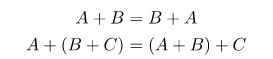
If $A$ , $B$ , and $C$ are any matrices of the same size, then

In fact, if $A = \left[ a_{ij} \right]$ and $B = \left[ b_{ij} \right]$ , then the $(i, j)$ -entries of $A + B$ and $B + A$ are, respectively, $a_{ij} + b_{ij}$ and $b_{ij} + a_{ij}$ . Since these are equal for all $i$ and $j$ , we get

$\begin{equation*} A + B = \left[ \begin{array}{c} a_{ij} + b_{ij} \end{array} \right] = \left[ \begin{array}{c} b_{ij} + a_{ij} \end{array} \right] = B + A \end{equation*}$

The associative law is verified similarly.

The $m \times n$ matrix in which every entry is zero is called the $m \times n$ zero matrix and is denoted as $0$ (or $0_{mn}$ if it is important to emphasize the size). Hence,

$\begin{equation*} 0 + X = X \end{equation*}$

holds for all $m \times n$ matrices $X$ . The negative of an $m \times n$ matrix $A$ (written $-A$ ) is defined to be the $m \times n$ matrix obtained by multiplying each entry of $A$ by $-1$ . If $A = \left[ a_{ij} \right]$ , this becomes $-A = \left[ -a_{ij} \right]$ . Hence,

$\begin{equation*} A + (-A) = 0 \end{equation*}$

holds for all matrices $A$ where, of course, $0$ is the zero matrix of the same size as $A$ .

A closely related notion is that of subtracting matrices. If $A$ and $B$ are two $m \times n$ matrices, their difference $A - B$ is defined by

$\begin{equation*} A - B = A + (-B) \end{equation*}$

Note that if $A = \left[ a_{ij} \right]$ and $B = \left[ b_{ij} \right]$ , then

$\begin{equation*} A - B = \left[ a_{ij} \right] + \left[ -b_{ij} \right] = \left[ a_{ij} - b_{ij} \right] \end{equation*}$

is the $m \times n$ matrix formed by subtracting corresponding entries.

Example 4 :

Let $A = \left[ \begin{array}{rrr} 3 & -1 & 0 \\ 1 & 2 & -4 \end{array} \right]$ , $B = \left[ \begin{array}{rrr} 1 & -1 & 1 \\ -2 & 0 & 6 \end{array} \right]$ , $C = \left[ \begin{array}{rrr} 1 & 0 & -2 \\ 3 & 1 & 1 \end{array} \right]$ .

Compute $-A$ , $A - B$ , and $A + B - C$ .

Solution:

$\begin{align*} -A &= \left[ \begin{array}{rrr} -3 & 1 & 0 \\ -1 & -2 & 4 \end{array} \right] \\ A - B &= \left[ \begin{array}{lcr} 3 - 1 & -1 - (-1) & 0 - 1 \\ 1 - (-2) & 2 - 0 & -4 - 6 \end{array} \right] = \left[ \begin{array}{rrr} 2 & 0 & -1 \\ 3 & 2 & -10 \end{array} \right] \\ A + B - C &= \left[ \begin{array}{rrl} 3 + 1 - 1 & -1 - 1 - 0 & 0 + 1 -(-2) \\ 1 - 2 - 3 & 2 + 0 - 1 & -4 + 6 -1 \end{array} \right] = \left[ \begin{array}{rrr} 3 & -2 & 3 \\ -4 & 1 & 1 \end{array} \right] \end{align*}$

Example 5 :Solve

$\left[ \begin{array}{rr} 3 & 2 \\ -1 & 1 \end{array} \right] + X = \left[ \begin{array}{rr} 1 & 0 \\ -1 & 2 \end{array} \right]$
where $X$ is a matrix.

We solve a numerical equation $a + x = b$ by subtracting the number $a$ from both sides to obtain $x = b - a$ . This also works for matrices. To solve
$\left[ \begin{array}{rr} 3 & 2 \\ -1 & 1 \end{array} \right] + X = \left[ \begin{array}{rr} 1 & 0 \\ -1 & 2 \end{array} \right]$
simply subtract the matrix
$\left[ \begin{array}{rr} 3 & 2 \\ -1 & 1 \end{array} \right]$
from both sides to get

$\begin{equation*} X = \left[ \begin{array}{rr} 1 & 0 \\ -1 & 2 \end{array} \right]- \left[ \begin{array}{rr} 3 & 2 \\ -1 & 1 \end{array} \right] = \left[ \begin{array}{cr} 1 - 3 & 0 - 2 \\ -1 - (-1) & 2 - 1 \end{array} \right] = \left[ \begin{array}{rr} -2 & -2 \\ 0 & 1 \end{array} \right] \end{equation*}$

The reader should verify that this matrix $X$ does indeed satisfy the original equation.

The solution in Example 2.1.5 solves the single matrix equation $A + X = B$ directly via matrix subtraction: $X = B - A$ . This ability to work with matrices as entities lies at the heart of matrix algebra.

It is important to note that the sizes of matrices involved in some calculations are often determined by the context. For example, if

$\begin{equation*} A + C = \left[ \begin{array}{rrr} 1 & 3 & -1 \\ 2 & 0 & 1 \end{array} \right] \end{equation*}$

then $A$ and $C$ must be the same size (so that $A + C$ makes sense), and that size must be $2 \times 3$ (so that the sum is $2 \times 3$ ). For simplicity we shall often omit reference to such facts when they are clear from the context.

Scalar Multiplication

In gaussian elimination, multiplying a row of a matrix by a number $k$ means multiplying every entry of that row by $k$ .

More generally, if $A$ is any matrix and $k$ is any number, the scalar multiple $kA$ is the matrix obtained from $A$ by multiplying each entry of $A$ by $k$ .

The term scalar arises here because the set of numbers from which the entries are drawn is usually referred to as the set of scalars. We have been using real numbers as scalars, but we could equally well have been using complex numbers.

Example 1 :

If $A = \left[ \begin{array}{rrr} 3 & -1 & 4 \\ 2 & 0 & 1 \end{array} \right]$
and $B = \left[ \begin{array}{rrr} 1 & 2 & -1 \\ 0 & 3 & 2 \end{array} \right],$
compute $5A$ , $\frac{1}{2}B$ , and $3A - 2B$ .

Solution:

$\begin{align*} 5A &= \left[ \begin{array}{rrr} 15 & -5 & 20 \\ 10 & 0 & 30 \end{array} \right], \quad \frac{1}{2}B = \left[ \begin{array}{rrr} \frac{1}{2} & 1 & -\frac{1}{2} \\ 0 & \frac{3}{2} & 1 \end{array} \right] \\ 3A - 2B &= \left[ \begin{array}{rrr} 9 & -3 & 12 \\ 6 & 0 & 18 \end{array} \right] - \left[ \begin{array}{rrr} 2 & 4 & -2 \\ 0 & 6 & 4 \end{array} \right] = \left[ \begin{array}{rrr} 7 & -7 & 14 \\ 6 & -6 & 14 \end{array} \right] \end{align*}$

If $A$ is any matrix, note that $kA$ is the same size as $A$ for all scalars $k$ . We also have

$\begin{equation*} 0A = 0 \quad \mbox{ and } \quad k0 = 0 \end{equation*}$

because the zero matrix has every entry zero. In other words, $kA = 0$ if either $k = 0$ or $A = 0$ . The converse of this statement is also true, as Example 2.1.7 shows.

Example 1 :

If $kA = 0$ , show that either $k = 0$ or $A = 0$ .

Solution:

Write $A = \left[ a_{ij} \right]$ so that $kA = 0$ means $ka_{ij} = 0$ for all $i$ and $j$ . If $k = 0$ , there is nothing to do. If $k \neq 0$ , then $ka_{ij} = 0$ implies that $a_{ij} = 0$ for all $i$ and $j$ ; that is, $A = 0$ .

Theorem

Let $A$ , $B$ , and $C$ denote arbitrary $m \times n$ matrices where $m$ and $n$ are fixed. Let $k$ and $p$ denote arbitrary real numbers. Then

$A + B = B + A$ .
$A + (B + C) = (A + B) + C$ .
There is an $m \times n$ matrix $0$ , such that $0 + A = A$ for each $A$ .
For each $A$ there is an $m \times n$ matrix, $-A$ , such that $A + (-A) = 0$ .
$k(A + B) = kA + kB$ .
$(k + p)A = kA + pA$ .
$(kp)A = k(pA)$ .
$1A = A$ .

Proof:
Properties 1–4 were given previously. To check Property 5, let $A = \left[ a_{ij} \right]$ and $B = \left[ b_{ij} \right]$ denote matrices of the same size. Then $A + B = \left[ a_{ij} + b_{ij} \right]$ , as before, so the $(i, j)$ -entry of $k(A + B)$ is

$\begin{equation*} k(a_{ij} + b_{ij}) = ka_{ij} + kb_{ij} \end{equation*}$

But this is just the $(i, j)$ -entry of $kA + kB$ , and it follows that $k(A + B) = kA + kB$ . The other Properties can be similarly verified; the details are left to the reader.

The Properties in Theorem 2.1.1 enable us to do calculations with matrices in much the same way that
numerical calculations are carried out. To begin, Property 2 implies that the sum

$\begin{equation*} (A + B) + C = A + (B + C) \end{equation*}$

is the same no matter how it is formed and so is written as $A + B + C$ . Similarly, the sum

$\begin{equation*} A + B + C + D \end{equation*}$

is independent of how it is formed; for example, it equals both $(A + B) + (C + D)$ and $A + \left[ B + (C + D) \right]$ . Furthermore, property 1 ensures that, for example,

$\begin{equation*} B + D + A + C = A + B + C + D \end{equation*}$

In other words, the order in which the matrices are added does not matter. A similar remark applies to sums of five (or more) matrices.

Properties 5 and 6 in Theorem 2.1.1 are called distributive laws for scalar multiplication, and they extend to sums of more than two terms. For example,

$\begin{equation*} k(A + B - C) = kA + kB - kC \end{equation*}$

$\begin{equation*} (k + p - m)A = kA + pA -mA \end{equation*}$

Similar observations hold for more than three summands. These facts, together with properties 7 and 8, enable us to simplify expressions by collecting like terms, expanding, and taking common factors in exactly the same way that algebraic expressions involving variables and real numbers are manipulated. The following example illustrates these techniques.

Example 1 :

Simplify $2(A + 3C) - 3(2C - B) - 3 \left[ 2(2A + B - 4C) - 4(A - 2C) \right]$ where $A, B$ and $C$ are all matrices of the same size.

Solution:

The reduction proceeds as though $A$ , $B$ , and $C$ were variables.

$\begin{align*} 2(A &+ 3C) - 3(2C - B) - 3 \left[ 2(2A + B - 4C) - 4(A - 2C) \right] \\ &= 2A + 6C - 6C + 3B - 3 \left[ 4A + 2B - 8C - 4A + 8C \right] \\ &= 2A + 3B - 3 \left[ 2B \right] \\ &= 2A - 3B \end{align*}$

Transpose of a Matrix

Many results about a matrix $A$ involve the rows of $A$ , and the corresponding result for columns is derived in an analogous way, essentially by replacing the word row by the word column throughout. The following definition is made with such applications in mind.

If $A$ is an $m \times n$ matrix, the transpose of $A$ , written $A^{T}$ , is the $n \times m$ matrix whose rows are just the columns of $A$ in the same order.

In other words, the first row of $A^{T}$ is the first column of $A$ (that is it consists of the entries of column 1 in order). Similarly the second row of $A^{T}$ is the second column of $A$ , and so on.

Write down the transpose of each of the following matrices.

$\begin{equation*} A = \left[ \begin{array}{r} 1 \\ 3 \\ 2 \end{array} \right] \quad B = \left[ \begin{array}{rrr} 5 & 2 & 6 \end{array} \right] \quad C = \left[ \begin{array}{rr} 1 & 2 \\ 3 & 4 \\ 5 & 6 \end{array} \right] \quad D = \left[ \begin{array}{rrr} 3 & 1 & -1 \\ 1 & 3 & 2 \\ -1 & 2 & 1 \end{array} \right] \end{equation*}$

Solution:

$\begin{equation*} A^{T} = \left[ \begin{array}{rrr} 1 & 3 & 2 \end{array} \right],\ B^{T} = \left[ \begin{array}{r} 5 \\ 2 \\ 6 \end{array} \right],\ C^{T} = \left[ \begin{array}{rrr} 1 & 3 & 5 \\ 2 & 4 & 6 \end{array} \right], \mbox{ and } D^{T} = D. \end{equation*}$

If $A = \left[ a_{ij} \right]$ is a matrix, write $A^{T} = \left[ b_{ij} \right]$ . Then $b_{ij}$ is the $j$ th element of the $i$ th row of $A^{T}$ and so is the $j$ th element of the $i$ th column of $A$ . This means $b_{ij} = a_{ji}$ , so the definition of $A^{T}$ can be stated as follows:

$\begin{equation*} \mbox{If } A = \left[ a_{ij} \right] \mbox{, then } A^{T} = \left[ a_{ji} \right]. \end{equation*}$

This is useful in verifying the following properties of transposition.

Theorem :

Let $A$ and $B$ denote matrices of the same size, and let $k$ denote a scalar.

If $A$ is an $m \times n$ matrix, then $A^{T}$ is an $n \times m$ matrix.
$(A^{T})^{T} = A$ .
$(kA)^{T} = kA^{T}$ .
$(A + B)^{T} = A^{T} + B^{T}$ .

Proof:

Property 1 is part of the definition of $A^{T}$ , and Property 2 follows from (2.1). As to Property 3: If $A = \leftB a_{ij} \rightB$ , then $kA = \leftB ka_{ij} \rightB$ , so (2.1) gives

$\begin{equation*} (kA)^{T} = \left[ ka_{ji} \right] = k \left[ a_{ji} \right] = kA^{T} \end{equation*}$

Finally, if $B = \left[ b_{ij} \right]$ , then $A + B = \left[ c_{ij} \right]$ where $c_{ij} = a_{ij} + b_{ij}$ Then (2.1) gives Property 4:

$\begin{equation*} (A + B)^{T} = \left[ c_{ij} \right]^{T} = \left[ c_{ji} \right] = \left[ a_{ji} + b_{ji} \right] = \left[ a_{ji} \right] + \left[ b_{ji} \right] = A^{T} + B^{T} \end{equation*}$

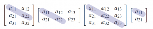
There is another useful way to think of transposition. If $A = \left[ a_{ij} \right]$ is an $m \times n$ matrix, the elements $a_{11}, a_{22}, a_{33}, \dots$ are called the main diagonal of $A$ . Hence the main diagonal extends down and to the right from the upper left corner of the matrix $A$ ; it is shaded in the following examples:

Thus forming the transpose of a matrix $A$ can be viewed as “flipping” $A$ about its main diagonal, or as “rotating” $A$ through $180^{\circ}$ about the line containing the main diagonal. This makes Property 2 in Theorem~?? transparent.

Example :

Solve for $A$ if $\left(2A^{T} - 3 \left[ \begin{array}{rr} 1 & 2 \\ -1 & 1 \end{array} \right] \right)^{T} = \left[ \begin{array}{rr} 2 & 3 \\ -1 & 2 \end{array} \right]$ .

Solution:

Using Theorem 2.1.2, the left side of the equation is

$\begin{equation*} \left(2A^{T} - 3 \left[ \begin{array}{rr} 1 & 2 \\ -1 & 1 \end{array} \right]\right)^{T} = 2\left(A^{T}\right)^{T} - 3 \left[ \begin{array}{rr} 1 & 2 \\ -1 & 1 \end{array} \right]^{T} = 2A - 3 \left[ \begin{array}{rr} 1 & -1 \\ 2 & 1 \end{array} \right] \end{equation*}$

Hence the equation becomes

$\begin{equation*} 2A - 3 \left[ \begin{array}{rr} 1 & -1 \\ 2 & 1 \end{array} \right] = \left[ \begin{array}{rr} 2 & 3 \\ -1 & 2 \end{array} \right] \end{equation*}$

Thus
$2A = \left[ \begin{array}{rr} 2 & 3 \\ -1 & 2 \end{array} \right] + 3 \left[ \begin{array}{rr} 1 & -1 \\ 2 & 1 \end{array} \right] = \left[ \begin{array}{rr} 5 & 0 \\ 5 & 5 \end{array} \right]$ , so finally
$A = \frac{1}{2} \left[ \begin{array}{rr} 5 & 0 \\ 5 & 5 \end{array} \right] = \frac{5}{2} \left[ \begin{array}{rr} 1 & 0 \\ 1 & 1 \end{array} \right]$ .

Note that Example 2.1.10 can also be solved by first transposing both sides, then solving for $A^{T}$ , and so obtaining $A = (A^{T})^{T}$ . The reader should do this.

The matrix $D = \left[ \begin{array}{rr} 1 & 2 \\ 2 & 5 \end{array}\right]$ in Example 2.1.9 has the property that $D = D^{T}$ . Such matrices are important; a matrix $A$ is called symmetric if $A = A^{T}$ . A symmetric matrix $A$ is necessarily square (if $A$ is $m \times n$ , then $A^{T}$ is $n \times m$ , so $A = A^{T}$ forces $n = m$ ). The name comes from the fact that these matrices exhibit a symmetry about the main diagonal. That is, entries that are directly across the main diagonal from each other are equal.

For example, $\left[ \begin{array}{ccc} a & b & c \\ b^\prime & d & e \\ c^\prime & e^\prime & f \end{array} \right]$ is symmetric when $b = b^\prime$ , $c = c^\prime$ , and $e = e^\prime$ .

Example :

If $A$ and $B$ are symmetric $n \times n$ matrices, show that $A + B$ is symmetric.

Solution:

We have $A^{T} = A$ and $B^{T} = B$ , so, by Theorem 2.1.2, we have $(A + B)^{T} = A^{T} + B^{T} = A + B$ . Hence $A + B$ is symmetric.

Example :

Suppose a square matrix $A$ satisfies $A = 2A^{T}$ . Show that necessarily $A = 0$ .

Solution:

If we iterate the given equation, Theorem 2.1.2 gives

$\begin{equation*} A = 2A^{T} = 2 {\left[ 2A^{T} \right]}^T = 2 \left[ 2(A^{T})^{T} \right] = 4A \end{equation*}$

Subtracting $A$ from both sides gives $3A = 0$ , so $A = \frac{1}{3}(0) = 0$ .

Matrix-Vector Multiplication

Up to now we have used matrices to solve systems of linear equations by manipulating the rows of the augmented matrix. In this section we introduce a different way of describing linear systems that makes more use of the coefficient matrix of the system and leads to a useful way of “multiplying” matrices.

Vectors

It is a well-known fact in analytic geometry that two points in the plane with coordinates $(a_{1}, a_{2})$ and $(b_{1}, b_{2})$ are equal if and only if $a_{1} = b_{1}$ and $a_{2} = b_{2}$ . Moreover, a similar condition applies to points $(a_{1}, a_{2}, a_{3})$ in space. We extend this idea as follows.

An ordered sequence $(a_{1}, a_{2}, \dots, a_{n})$ of real numbers is called an ordered $\bm{n}$ –tuple. The word “ordered” here reflects our insistence that two ordered $n$ -tuples are equal if and only if corresponding entries are the same. In other words,

$\begin{equation*} (a_{1}, a_{2}, \dots, a_{n}) = (b_{1}, b_{2}, \dots, b_{n}) \quad \mbox{if and only if} \quad a_{1} = b_{1}, a_{2} = b_{2}, \dots, \mbox{ and } a_{n} = b_{n}. \end{equation*}$

Thus the ordered $2$ -tuples and $3$ -tuples are just the ordered pairs and triples familiar from geometry.

Let $\mathbb{R}$ denote the set of all real numbers. The set of all ordered $n$ -tuples from $\mathbb{R}$ has a special notation:

$\begin{equation*} \mathbb{R}^{n} \mbox{ denotes the set of all ordered }n\mbox{-tuples of real numbers.} \end{equation*}$

There are two commonly used ways to denote the $n$ -tuples in $\mathbb{R}^{n}$ : As rows $(r_{1}, r_{2}, \dots, r_{n})$ or columns $\left[ \begin{array}{c} r_{1} \\ r_{2} \\ \vdots \\ r_{n} \end{array} \right]$ ;

the notation we use depends on the context. In any event they are called vectors or $n$ –vectors and will be denoted using bold type such as x or v. For example, an $m \times n$ matrix $A$ will be written as a row of columns:

$\begin{equation*} A = \left[ \begin{array}{cccc} \textbf{a}_{1} & \textbf{a}_{2} & \cdots & \textbf{a}_{n} \end{array} \right] \mbox{ where } \textbf{a}_{j} \mbox{ denotes column } j \mbox{ of } A \mbox{ for each } j. \end{equation*}$

If $\textbf{x}$ and $\textbf{y}$ are two $n$ -vectors in $\mathbf{R}^n$ , it is clear that their matrix sum $\textbf{x} + \textbf{y}$ is also in $\mathbf{R}^n$ as is the scalar multiple $k\textbf{x}$ for any real number $k$ . We express this observation by saying that $\mathbf{R}^n$ is closed under addition and scalar multiplication. In particular, all the basic properties in Theorem 2.1.1 are true of these $n$ -vectors. These properties are fundamental and will be used frequently below without comment. As for matrices in general, the $n \times 1$ zero matrix is called the zero $\bm{n}$ –vector in $\mathbf{R}^n$ and, if $\textbf{x}$ is an $n$ -vector, the $n$ -vector $-\textbf{x}$ is called the negative $\textbf{x}$ .

Of course, we have already encountered these $n$ -vectors in Section 1.3 as the solutions to systems of linear equations with $n$ variables. In particular we defined the notion of a linear combination of vectors and showed that a linear combination of solutions to a homogeneous system is again a solution. Clearly, a linear combination of $n$ -vectors in $\mathbf{R}^n$ is again in $\mathbf{R}^n$ , a fact that we will be using.

Matrix-Vector Multiplication

Given a system of linear equations, the left sides of the equations depend only on the coefficient matrix $A$ and the column $\textbf{x}$ of variables, and not on the constants. This observation leads to a fundamental idea in linear algebra: We view the left sides of the equations as the “product” $A\textbf{x}$ of the matrix $A$ and the vector $\textbf{x}$ . This simple change of perspective leads to a completely new way of viewing linear systems—one that is very useful and will occupy our attention throughout this book.

To motivate the definition of the “product” $A\textbf{x}$ , consider first the following system of two equations in three variables:

(2.2) $\begin{equation*} \arraycolsep=1pt \begin{array}{rrrrrrr} ax_{1} & + & bx_{2} & + & cx_{3} & = & b_{1} \\ a^{\prime}x_{1} & + & b^{\prime}x_{2} & + & c^{\prime}x_{3} & = & b_{1} \end{array} \end{equation*}$

and let $A = \left[ \begin{array}{ccc} a & b & c \\ a^\prime & b^\prime & c^\prime \end{array} \right]$ , $\textbf{x} = \left[ \begin{array}{c} x_{1} \\ x_{2} \\ x_{3} \end{array} \right]$ , $\textbf{b} = \left[ \begin{array}{c} b_{1} \\ b_{2} \end{array} \right]$ denote the coefficient matrix, the variable matrix, and the constant matrix, respectively. The system (2.2) can be expressed as a single vector equation

$\begin{equation*} \left[ \arraycolsep=1pt \begin{array}{rrrrr} ax_{1} & + & bx_{2} & + & cx_{3} \\ a^\prime x_{1} & + & b^\prime x_{2} & + & c^\prime x_{3} \end{array} \right] = \left[ \begin{array}{c} b_{1} \\ b_{2} \end{array} \right] \end{equation*}$

which in turn can be written as follows:

$\begin{equation*} x_{1} \left[ \begin{array}{c} a \\ a^\prime \end{array} \right] + x_{2} \left[ \begin{array}{c} b \\ b^\prime \end{array} \right] + x_{3} \left[ \begin{array}{c} c \\ c^\prime \end{array} \right] = \left[ \begin{array}{c} b_{1} \\ b_{2} \end{array} \right] \end{equation*}$

Now observe that the vectors appearing on the left side are just the columns

$\begin{equation*} \textbf{a}_{1} = \left[ \begin{array}{c} a \\ a^\prime \end{array} \right], \textbf{a}_{2} = \left[ \begin{array}{c} b \\ b^\prime \end{array} \right], \mbox{ and } \textbf{a}_{3} = \left[ \begin{array}{c} c \\ c^\prime \end{array} \right] \end{equation*}$

of the coefficient matrix $A$ . Hence the system (2.2) takes the form

(2.3) $\begin{equation*} x_{1}\textbf{a}_{1} + x_{2}\textbf{a}_{2} + x_{3}\textbf{a}_{3} = \textbf{b} \end{equation*}$

This shows that the system (2.2) has a solution if and only if the constant matrix $\textbf{b}$ is a linear combination of the columns of $A$ , and that in this case the entries of the solution are the coefficients $x_{1}$ , $x_{2}$ , and $x_{3}$ in this linear combination.

Moreover, this holds in general. If $A$ is any $m \times n$ matrix, it is often convenient to view $A$ as a row of columns. That is, if $\textbf{a}_{1}, \textbf{a}_{2}, \dots, \textbf{a}_{n}$ are the columns of $A$ , we write

$\begin{equation*} A = \left[ \begin{array}{cccc} \textbf{a}_{1} & \textbf{a}_{2} & \cdots & \textbf{a}_{n} \end{array} \right] \end{equation*}$

and say that $A = \left[ \begin{array}{cccc}\textbf{a}_{1} & \textbf{a}_{2} & \cdots & \textbf{a}_{n} \end{array} \right]$ is given in terms of its columns.

Now consider any system of linear equations with $m \times n$ coefficient matrix $A$ . If $\textbf{b}$ is the constant matrix of the system, and if $\textbf{x} = \left[ \begin{array}{c} x_{1} \\ x_{2} \\ \vdots \\ x_{n} \end{array} \right]$
is the matrix of variables then, exactly as above, the system can be written as a single vector equation

(2.4) $\begin{equation*} x_{1}\textbf{a}_{1} + x_{2}\textbf{a}_{2} + \dots + x_{n}\textbf{a}_{n} = \textbf{b} \end{equation*}$

Write the system
$\left\lbrace \arraycolsep=1pt \begin{array}{rrrrrrr} 3x_{1} & + & 2x_{2} & - & 4x_{3} & = & 0 \\ x_{1} & - & 3x_{2} & + & x_{3} & = & 3 \\ & & x_{2} & - & 5x_{3} & = & -1 \end{array} \right.$
in the form given in (2.4).

Solution:

$\begin{equation*} x_{1} \left[ \begin{array}{r} 3 \\ 1 \\ 0 \end{array} \right] + x_{2} \left[ \begin{array}{r} 2 \\ -3 \\ 1 \end{array} \right] + x_{3} \left[ \begin{array}{r} -4 \\ 1 \\ -5 \end{array} \right] = \left[ \begin{array}{r} 0 \\ 3 \\ -1 \end{array} \right] \end{equation*}$

As mentioned above, we view the left side of (2.4) as the product of the matrix $A$ and the vector $\textbf{x}$ . This basic idea is formalized in the following definition:

Let $A = \left[ \begin{array}{cccc} \textbf{a}_{1} &\textbf{a}_{2} & \cdots & \textbf{a}_{n} \end{array} \right]$ be an $m \times n$ matrix, written in terms of its columns $\textbf{a}_{1}, \textbf{a}_{2}, \dots, \textbf{a}_{n}$ . If $\textbf{x} = \left[ \begin{array}{c} x_{1} \\ x_{2} \\ \vdots \\ x_{n} \end{array} \right]$
is any n-vector, the product $A\textbf{x}$ is defined to be the $m$ -vector given by:

$\begin{equation*} A\textbf{x} = x_{1}\textbf{a}_{1} + x_{2}\textbf{a}_{2} + \cdots + x_{n}\textbf{a}_{n} \end{equation*}$

In other words, if $A$ is $m \times n$ and $\textbf{x}$ is an $n$ -vector, the product $A\textbf{x}$ is the linear combination of the columns of $A$ where the coefficients are the entries of $\textbf{x}$ (in order).

Note that if $A$ is an $m \times n$ matrix, the product $A\textbf{x}$ is only defined if $\textbf{x}$ is an $n$ -vector and then the vector $A\textbf{x}$ is an $m$ -vector because this is true of each column $\textbf{a}_{j}$ of $A$ . But in this case the system of linear equations with coefficient matrix $A$ and constant vector $\textbf{b}$ takes the form of a single matrix equation

$\begin{equation*} A\textbf{x} = \textbf{b} \end{equation*}$

The following theorem combines Definition 2.5 and equation (2.4) and summarizes the above discussion. Recall that a system of linear equations is said to be consistent if it has at least one solution.

Theorem :

Every system of linear equations has the form $A\textbf{x} = \textbf{b}$ where $A$ is the coefficient matrix, $\textbf{b}$ is the constant matrix, and $\textbf{x}$ is the matrix of variables.
The system $A\textbf{x} = \textbf{b}$ is consistent if and only if $\textbf{b}$ is a linear combination of the columns of $A$ .
If $\textbf{a}_{1}, \textbf{a}_{2}, \dots, \textbf{a}_{n}$ are the columns of $A$ and if $\textbf{x} = \left[ \begin{array}{c} x_{1} \\ x_{2} \\ \vdots \\ x_{n} \end{array} \right]$ , then $\textbf{x}$ is a solution to the linear system $A\textbf{x} = \textbf{b}$ if and only if $x_{1}, x_{2}, \dots, x_{n}$ are a solution of the vector equation
$\begin{equation*} x_{1}\textbf{a}_{1} + x_{2}\textbf{a}_{2} + \cdots + x_{n}\textbf{a}_{n} = \textbf{b} \end{equation*}$

A system of linear equations in the form $A\textbf{x} = \textbf{b}$ as in (1) of Theorem 2.2.1 is said to be written in matrix form. This is a useful way to view linear systems as we shall see.

Theorem 2.2.1 transforms the problem of solving the linear system $A\textbf{x} = \textbf{b}$ into the problem of expressing the constant matrix $B$ as a linear combination of the columns of the coefficient matrix $A$ . Such a change in perspective is very useful because one approach or the other may be better in a particular situation; the importance of the theorem is that there is a choice.

Example :

If $A = \left[ \begin{array}{rrrr} 2 & -1 & 3 & 5 \\ 0 & 2 & -3 & 1 \\ -3 & 4 & 1 & 2 \end{array} \right]$ and
$\textbf{x} = \left[ \begin{array}{r} 2 \\ 1 \\ 0 \\ -2 \end{array} \right]$ , compute $A\textbf{x}$ .

Solution:

By Definition 2.5:
$A\textbf{x} = 2 \left[ \begin{array}{r} 2 \\ 0 \\ -3 \end{array} \right] + 1 \left[ \begin{array}{r} -1 \\ 2 \\ 4 \end{array} \right] + 0 \left[ \begin{array}{r} 3 \\ -3 \\ 1 \end{array} \right] - 2 \left[ \begin{array}{r} 5 \\ 1 \\ 2 \end{array} \right] = \left[ \begin{array}{r} -7 \\ 0 \\ -6 \end{array} \right]$ .

Example :

Given columns $\textbf{a}_{1}$ , $\textbf{a}_{2}$ , $\textbf{a}_{3}$ , and $\textbf{a}_{4}$ in $\mathbf{R}^3$ , write $2\textbf{a}_{1} - 3\textbf{a}_{2} + 5\textbf{a}_{3} + \textbf{a}_{4}$ in the form $A\textbf{x}$ where $A$ is a matrix and $\textbf{x}$ is a vector.

Solution:

Here the column of coefficients is
$\textbf{x} = \left[ \begin{array}{r} 2 \\ -3 \\ 5 \\ 1 \end{array} \right].$
Hence Definition 2.5 gives

$\begin{equation*} A\textbf{x} = 2\textbf{a}_{1} - 3\textbf{a}_{2} + 5\textbf{a}_{3} + \textbf{a}_{4} \end{equation*}$

where $A = \left[ \begin{array}{cccc} \textbf{a}_{1} & \textbf{a}_{2} & \textbf{a}_{3} & \textbf{a}_{4} \end{array} \right]$ is the matrix with $\textbf{a}_{1}$ , $\textbf{a}_{2}$ , $\textbf{a}_{3}$ , and $\textbf{a}_{4}$ as its columns.

Let $A = \left[ \begin{array}{cccc} \textbf{a}_{1} & \textbf{a}_{2} & \textbf{a}_{3} & \textbf{a}_{4} \end{array} \right]$ be the $3 \times 4$ matrix given in terms of its columns
$\textbf{a}_{1} = \left[ \begin{array}{r} 2 \\ 0 \\ -1 \end{array} \right]$ , $\textbf{a}_{2} = \left[ \begin{array}{r} 1 \\ 1 \\ 1 \end{array} \right]$ , $\textbf{a}_{3} = \left[ \begin{array}{r} 3 \\ -1 \\ -3 \end{array} \right]$ , and $\textbf{a}_{4} = \left[ \begin{array}{r} 3 \\ 1 \\ 0 \end{array} \right]$ .
In each case below, either express $\textbf{b}$ as a linear combination of $\textbf{a}_{1}$ , $\textbf{a}_{2}$ , $\textbf{a}_{3}$ , and $\textbf{a}_{4}$ , or show that it is not such a linear combination. Explain what your answer means for the corresponding system $A\textbf{x} = \textbf{b}$ of linear equations.

1. $\textbf{b} = \left[ \begin{array}{r} 1 \\ 2 \\ 3 \end{array} \right]$

2. $\textbf{b} = \left[ \begin{array}{r} 4 \\ 2 \\ 1 \end{array} \right]$

Solution:

By Theorem 2.2.1, $\textbf{b}$ is a linear combination of $\textbf{a}_{1}$ , $\textbf{a}_{2}$ , $\textbf{a}_{3}$ , and $\textbf{a}_{4}$ if and only if the system $A\textbf{x} = \textbf{b}$ is consistent (that is, it has a solution). So in each case we carry the augmented matrix $\left[ A|\textbft{b} \right]$ of the system $A\textbf{x} = \textbf{b}$ to reduced form.

1. Here
$\left[ \begin{array}{rrrr|r} 2 & 1 & 3 & 3 & 1 \\ 0 & 1 & -1 & 1 & 2 \\ -1 & 1 & -3 & 0 & 3 \end{array} \right] \rightarrow \left[ \begin{array}{rrrr|r} 1 & 0 & 2 & 1 & 0 \\ 0 & 1 & -1 & 1 & 0 \\ 0 & 0 & 0 & 0 & 1 \end{array} \right]$ , so the system $A\textbf{x} = \textbf{b}$ has no solution in this case. Hence $\textbf{b}$ is \textit{not} a linear combination of $\textbf{a}_{1}$ , $\textbf{a}_{2}$ , $\textbf{a}_{3}$ , and $\textbf{a}_{4}$ .

2. Now
$\left[ \begin{array}{rrrr|r} 2 & 1 & 3 & 3 & 4 \\ 0 & 1 & -1 & 1 & 2 \\ -1 & 1 & -3 & 0 & 1 \end{array} \right] \rightarrow \left[ \begin{array}{rrrr|r} 1 & 0 & 2 & 1 & 1 \\ 0 & 1 & -1 & 1 & 2 \\ 0 & 0 & 0 & 0 & 0 \end{array} \right]$ , so the system $A\textbf{x} = \textbf{b}$ is consistent.

Thus $\textbf{b}$ is a linear combination of $\textbf{a}_{1}$ , $\textbf{a}_{2}$ , $\textbf{a}_{3}$ , and $\textbf{a}_{4}$ in this case. In fact the general solution is $x_{1} = 1 - 2s - t$ , $x_{2} = 2 + s - t$ , $x_{3} = s$ , and $x_{4} = t$ where $s$ and $t$ are arbitrary parameters. Hence $x_{1}\textbf{a}_{1} + x_{2}\textbf{a}_{2} + x_{3}\textbf{a}_{3} + x_{4}\textbf{a}_{4} = \textbf{b} = \left[ \begin{array}{r} 4 \\ 2 \\ 1 \end{array} \right]$
for any choice of $s$ and $t$ . If we take $s = 0$ and $t = 0$ , this becomes $\textbf{a}_{1} + 2\textbf{a}_{2} = \textbf{b}$ , whereas taking $s = 1 = t$ gives $-2\textbf{a}_{1} + 2\textbf{a}_{2} + \textbf{a}_{3} + \textbf{a}_{4} = \textbf{b}$ .

Taking $A$ to be the zero matrix, we have $0\textbf{x} = \textbf{0}$ for all vectors $\textbf{x}$ by Definition 2.5 because every column of the zero matrix is zero. Similarly, $A\textbf{0} = \textbf{0}$ for all matrices $A$ because every entry of the zero vector is zero.

Example :

If $I = \left[ \begin{array}{rrr} 1 & 0 & 0 \\ 0 & 1 & 0 \\ 0 & 0 & 1 \end{array} \right]$ , show that $I\textbf{x} = \textbf{x}$ for any vector $\textbf{x}$ in $\mathbf{R}^3$ .

Solution:

If $\textbf{x} = \left[ \begin{array}{r} x_{1} \\ x_{2} \\ x_{3} \end{array} \right],$ then Definition 2.5 gives

$\begin{equation*} I\textbf{x} = x_{1} \left[ \begin{array}{r} 1 \\ 0 \\ 0 \\ \end{array} \right] + x_{2} \left[ \begin{array}{r} 0 \\ 1 \\ 0 \\ \end{array} \right] + x_{3} \left[ \begin{array}{r} 0 \\ 0 \\ 1 \\ \end{array} \right] = \left[ \begin{array}{r} x_{1} \\ 0 \\ 0 \\ \end{array} \right] + \left[ \begin{array}{r} 0 \\ x_{2} \\ 0 \\ \end{array} \right] + \left[ \begin{array}{r} 0 \\ 0 \\ x_{3} \\ \end{array} \right] = \left[ \begin{array}{r} x_{1} \\ x_{2} \\ x_{3} \\ \end{array} \right] = \textbf{x} \end{equation*}$

The matrix $I$ in Example 2.2.6 is called the $3 \times 3$ identity matrix, and we will encounter such matrices again in future. Before proceeding, we develop some algebraic properties of matrix-vector multiplication that are used extensively throughout linear algebra.

Theorem :

Let $A$ and $B$ be $m \times n$ matrices, and let $\vect{x}$ and $\vect{y}$ be $n$ -vectors in $\RR^n$ . Then:

$A(\textbf{x} + \textbf{y}) = A\textbf{x} + A\textbf{y}$ .
$A(a\textbf{x}) = a(A\textbf{x}) = (aA)\textbf{x}$ for all scalars $a$ .
$(A + B)\textbf{x} = A\textbf{x} + B\textbf{x}$ .

Proof:

We prove (3); the other verifications are similar and are left as exercises. Let $A = \left[ \begin{array}{cccc} \textbf{a}_{1} & \textbf{a}_{2} & \cdots & \textbf{a}_{n} \end{array} \right]$ and $B = \left[ \begin{array}{cccc} \textbf{b}_{1} & \textbf{b}_{2} & \cdots & \textbf{b}_{n} \end{array} \right]$ be given in terms of their columns. Since adding two matrices is the same as adding their columns, we have

$\begin{equation*} A + B = \left[ \begin{array}{cccc} \textbf{a}_{1} + \textbf{b}_{1} & \textbf{a}_{2} + \textbf{b}_{2} & \cdots & \textbf{a}_{n} + \textbf{b}_{n} \end{array} \right] \end{equation*}$

If we write $\textbf{x} = \left[ \begin{array}{c} x_{1} \\ x_{2} \\ \vdots \\ x_{n} \end{array} \right].$
Definition 2.5 gives

$\begin{align*} (A + B)\textbf{x} &= x_{1}(\textbf{a}_{1} + \textbf{b}_{1}) + x_{2}(\textbf{a}_{2} + \textbf{b}_{2}) + \dots + x_{n}(\textbf{a}_{n} + \textbf{b}_{n}) \\ &= (x_{1}\textbf{a}_{1} + x_{2}\textbf{a}_{2} + \dots + x_{n}\textbf{a}_{n}) + (x_{1}\textbf{b}_{1} + x_{2}\textbf{b}_{2} + \dots + x_{n}\textbf{b}_{n})\\ &= A\textbf{x} + B\textbf{x} \end{align*}$

Theorem 2.2.2 allows matrix-vector computations to be carried out much as in ordinary arithmetic. For example, for any $m \times n$ matrices $A$ and $B$ and any $n$ -vectors $\textbf{x}$ and $\textbf{y}$ , we have:

$\begin{equation*} A(2 \textbf{x} - 5 \textbf{y}) = 2A\textbf{x} - 5A\textbf{y} \quad \mbox{ and } \quad (3A -7B)\textbf{x} = 3A\textbf{x} - 7B\textbf{x} \end{equation*}$

We will use such manipulations throughout the book, often without mention.

Thursday 23 June 2022

MathWithNaziaa : Matrices in Linear Algebra

Matrix Addition, Scalar Multiplication, and Transposition

Matrix Addition

Scalar Multiplication

Transpose of a Matrix

Matrix-Vector Multiplication

Vectors

Matrix-Vector Multiplication

No comments:

Post a Comment