
Calculus, branch of mathematics concerned with the
calculation of instantaneous rates of change (differential calculus) and
the summation of infinitely many small factors to determine some whole (integral
calculus). Two mathematicians, Isaac Newton of England and Gottfried
Wilhelm Leibniz of Germany, share credit for having independently developed
the calculus in the 17th century. Calculus is now the basic entry point for
anyone wishing to study physics, chemistry, biology, economics,
finance, or actuarial science. Calculus makes it possible to solve
problems as diverse as tracking the position of a space shuttle
or predicting the pressure building up behind a dam as the water rises.
Computers have become a valuable tool for solving calculus problems that were
once considered impossibly difficult.
Calculus is used in a multitude of fields that you
wouldn't ordinarily think would make use of its concepts. Among them are
physics, engineering, economics, statistics, and medicine. Calculus is also
used in such disparate areas as space travel, as well as determining how
medications interact with the body, and even how to build safer
structures. You'll understand why calculus is useful in so many areas if
you know a bit about its history as well as what it is designed to do and
measure.
Calculus
is concerned with two basic operations, differentiation and integration, and is
a tool used by engineers to determine such quantities as rates of change and
areas; in fact, calculus is the mathematical ‘backbone’ for dealing with
problems where variables change with time or some other reference variable and
a basic understanding of calculus is essential for further study and the
development of confidence in solving practical engineering problems. This will
become evident in the next chapter where physical systems will be modelled and
the use of ‘rates of change’ equations (called differential equations) will
allow the physical system to be represented, an analysis made and a solution
formed under defined conditions. This chapter is an introduction to the techniques
of calculus and a consideration of some of their engineering applications. The
topic continues in the next chapter with a discussion of the use of
differential equations to represent physical systems and their solution for
various inputs.
A good understanding of Calculus requires you to have a basic knowledge of:
Functions
These functions are further characterized as
- Polynomials
- Rational
Functions
- Logarithms
- Exponentials
- Trigonometric
Throughout this course, we will be making use of these terms frequently, so
it is better if you have a good understanding of the terms listed above. These
are not very difficult-to-understand concepts. You may study them on your own
before you proceed further into learning concepts of Calculus. Next we move to
the core concepts and examples of Calculus.
Polynomials
A polynomial function has the form
are real numbers and n is a nonnegative integer. In other words, a
polynomial is the sum of one or more monomials with real coefficients and
non-negative integer exponents. The degree of the polynomial function is the
highest value for n where n is not equal to 0.
Polynomial functions of only one term are called monomials or power functions. A power function has the form
is called a root of the function f. When a polynomial function is completely factored, each of the factors helps identify zeros of the function.
Rational Functions
Rational function" is the name given to a function which can be represented as the quotient of polynomials, just as a rational number is a number which can be expressed as a quotient of whole numbers. Rational functions supply important examples and occur naturally in many contexts. All polynomials are rational functions.
Logarithms
and `log(x/y)=log x - log y are logarithmic functions that essentially simplify multiplication to addition and division to subtraction. Logarithmic functions are the inverse of their exponential counterparts.
Exponentials
An exponential function is a mathematical function of the following form:
where x is a variable, and a is a constant called the base of the function. The most commonly encountered exponential-function base is the transcendental number e , which is equal to approximately 2.71828. Thus, the above expression becomes:
When the exponent in this function increases by 1, the value of the function increases by a factor of e . When the exponent decreases by 1, the value of the function decreases by this same factor (it is divided by e ).
Trigonometric
A function of an angle expressed as the ratio of two of the sides of a right
triangle that contains that angle; the sine, cosine, tangent, cotangent,
secant, and cosecant. Also called circular function.
The roots of calculus lie in some of
the oldest geometry problems on record. The Egyptian Rhind papyrus
(c. 1650 bce) gives rules for finding the area of a circle and
the volume of a truncated pyramid. Ancient Greek geometers investigated finding
tangents to curves, the centre of gravity of plane and solid figures,
and the volumes of objects formed by revolving various curves about a fixed
axis.
By 1635 the Italian mathematician Bonaventura
Cavalieri had supplemented the rigorous tools of Greek geometry with heuristic
methods that used the idea of infinitely small segments of lines, areas, and
volumes. In 1637 the French mathematician-philosopher René
Descartes published his invention of analytic geometry for giving algebraic
descriptions of geometric figures. Descartes’s method, in combination with an
ancient idea of curves being generated by a moving point, allowed
mathematicians such as Newton to describe motion algebraically. Suddenly
geometers could go beyond the single cases and ad hoc methods of previous
times. They could see patterns of results, and so conjecture new results, that
the older geometric language had obscured.
For example, the Greek geometer Archimedes
(287–212/211 bce) discovered as an isolated
result that the area of a segment of a parabola is equal to a certain triangle.
But with algebraic notation, in which a parabola is written as y = x2,
Cavalieri and other geometers soon noted that the area between this curve and
the x-axis from 0 to a is a3/3 and that a
similar rule holds for the curve y = x3—namely,
that the corresponding area is a4/4. From here it was not
difficult for them to guess that the general formula for the area under a curve
y = xn is an + 1/(n + 1).
The problem of finding tangents to curves was closely
related to an important problem that arose from the Italian scientist Galileo
Galilei’s investigations of motion, that of finding the velocity
at any instant of a particle moving according to some law. Galileo established
that in t seconds a freely falling body falls a distance gt2/2,
where g is a constant (later interpreted by Newton as the gravitational
constant). With the definition of average velocity as the distance per time,
the body’s average velocity over an interval from t to t + h
is given by the expression [g(t + h)2/2 − gt2/2]/h.
This simplifies to gt + gh/2 and is called the difference quotient of the function gt2/2.
As h approaches 0, this formula approaches gt, which is
interpreted as the instantaneous velocity of a falling body at time t.
This expression for motion is identical to that
obtained for the slope of the tangent to the parabola f(t) =
y = gt2/2 at the point t. In
this geometric context, the expression gt + gh/2
(or its equivalent [f(t + h) − f(t)]/h)
denotes the slope of a secant line connecting the point (t, f(t))
to the nearby point (t + h, f(t + h))
(see figure).
In the limit, with smaller and smaller intervals h, the secant line
approaches the tangent line and its slope at the point t.
Thus, the difference quotient can be interpreted as
instantaneous velocity or as the slope of a tangent to a curve. It was the
calculus that established this deep connection between geometry and physics—in
the process transforming physics and giving a new impetus to the study of
geometry.
Differentiation and integration
Independently, Newton and Leibniz established simple
rules for finding the formula for the slope of the tangent to a curve at any
point on it, given only a formula for the curve. The rate of change of a
function f (denoted by f′) is known as its derivative.
Finding the formula of the derivative function is called differentiation,
and the rules for doing so form the basis of differential calculus. Depending
on the context, derivatives may be interpreted as slopes of tangent lines,
velocities of moving particles, or other quantities, and therein lies the great
power of the differential calculus.
An important application of differential calculus is
graphing a curve given its equation y = f(x).
This involves, in particular, finding local maximum and minimum points on the graph,
as well as changes in inflection (convex to concave, or vice versa). When
examining a function used in a mathematical model, such geometric notions have
physical interpretations that allow a scientist or engineer to quickly gain a
feeling for the behaviour of a physical system.
The other great discovery of Newton and Leibniz was
that finding the derivatives of functions was, in a precise sense, the inverse
of the problem of finding areas under curves—a principle now known as the fundamental theorem of calculus. Specifically, Newton
discovered that if there exists a function F(t) that denotes
the area under the curve y = f(x) from,
say, 0 to t, then this function’s derivative will equal the original
curve over that interval, F′(t) = f(t).
Hence, to find the area under the curve y = x2
from 0 to t, it is enough to find a function F so that F′(t) = t2.
The differential calculus shows that the most general such function is x3/3 + C,
where C is an arbitrary constant. This is called the (indefinite) integral of the function y = x2,
and it is written as ∫x2dx. The initial symbol ∫
is an elongated S, which stands for sum, and dx indicates an
infinitely small increment of the variable, or axis, over which the function is
being summed. Leibniz introduced this because he thought of integration
as finding the area under a curve by a summation of the areas of infinitely
many infinitesimally thin rectangles between the x-axis and the curve.
Newton and Leibniz discovered that integrating f(x) is
equivalent to solving a differential equation—i.e., finding a function F(t)
so that F′(t) = f(t). In physical
terms, solving this equation can be interpreted as finding the distance F(t)
traveled by an object whose velocity has a given expression f(t).
The branch of the calculus concerned with calculating integrals
is the integral calculus, and among its many applications are finding work done
by physical systems and calculating pressure behind a dam at a given depth.
Practical Applications
Calculus has many practical
applications in real life. Some of the concepts that use calculus include
motion, electricity, heat, light, harmonics, acoustics, and astronomy. Calculus
is used in geography, computer vision (such as for autonomous driving of cars),
photography, artificial intelligence, robotics, video games, and even movies.
Calculus is also used to calculate the rates of radioactive decay in chemistry,
and even to predict birth and death rates, as well as in the study of gravity
and planetary motion, fluid flow, ship design, geometric curves, and bridge
engineering.
In physics, for example, calculus is
used to help define, explain, and calculate motion, electricity, heat, light,
harmonics, acoustics, astronomy, and dynamics. Einstein's theory of relativity
relies on calculus, a field of mathematics that also helps economists predict
how much profit a company or industry can make. And in shipbuilding, calculus
has been used for many years to determine both the curve of the hull of the
ship (using differential calculus), as well as the area under the hull (using
integral calculus), and even in the general design of ships.
In addition, calculus is used to check
answers for different mathematical disciplines such as statistics, analytical
geometry, and algebra.
Calculus in Economics
Economists use calculus to predict supply,
demand, and maximum potential profits. Supply and demand are, after all,
essentially charted on a curve—and an ever-changing curve at that.
Economists use calculus to determine
the price elasticity of demand. They refer to the ever-changing
supply-and-demand curve as "elastic," and the actions of the curve as
"elasticity." To calculate an exact measure of elasticity at a
particular point on a supply or demand curve, you need to think about
infinitesimally small changes in price and, as a result, incorporate
mathematical derivatives into your elasticity formulas. Calculus allows you to
determine specific points on that ever-changing supply-and-demand curve.
The Fundamental Theorem of Calculus
In order to work our way towards understanding the fundamental theorem of
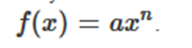
calculus, let’s revisit the car’s position and velocity example:
Line Plot of the Car’s Position Against Time

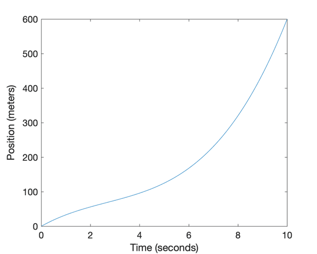
Line Plot of the Car’s Velocity Against Time
In computing the derivative we had solved the forward problem, where
we found the velocity from the slope of the position graph at any time, t.
But what if we would like to solve the backward problem, where we are
given the velocity graph, v(t), and wish to find the distance
travelled? The solution to this problem is to calculate the area under the
curve (the shaded region) up to time, t:
The Shaded Region is the Area Under the Curve
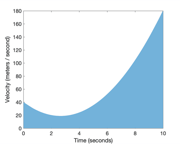
We do not have a specific formula to define the area of the shaded region
directly. But we can apply the mathematics of calculus to cut the shaded region
under the curve into many infinitely thin rectangles, for which we have a
formula:

Cutting the Shaded Region Into Many Rectangles of
Width, Δt
If we consider the ith rectangle, chosen arbitrarily to
span the time interval Δt, we can define its area as its length times
its width:
area_of_rectangle = v(ti)
Δti
We can have as many rectangles as necessary in order to span the interval of
interest, which in this case is the shaded region under the curve. For
simplicity, let’s denote this closed interval by [a, b]. Finding
the area of this shaded region (and, hence, the distance travelled), then
reduces to finding the sum of the n number of rectangles:
total_area = v(t0)
Δt0 + v(t1) Δt1
+ … + v(tn) Δtn
We can express this sum even more compactly by applying the Riemann sum with
sigma notation:

If we cut (or divide) the region under the curve by a finite number of
rectangles, then we find that the Riemann sum gives us an approximation of
the area, since the rectangles will not fit the area under the curve exactly.
If we had to position the rectangles so that their upper left or upper right
corners touch the curve, the Riemann sum gives us either an underestimate or an
overestimate of the true area, respectively. If the midpoint of each rectangle
had to touch the curve, then the part of the rectangle protruding above the
curve roughly compensates for the gap between the curve and neighbouring
rectangles:
Approximating the Area Under the Curve with Left Sums

Approximating the Area Under the Curve with Right Sums
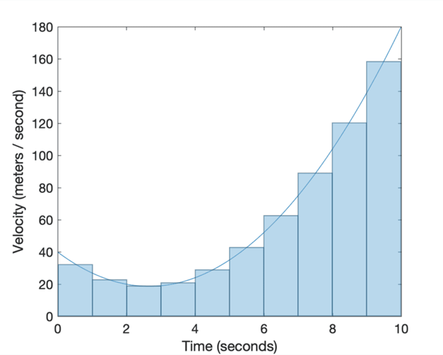
Approximating the Area Under the Curve with Midpoint
Sums
The solution to finding the exact area under the curve, is to reduce
the rectangles’ width so much that they become infinitely thin (recall
the Infinity Principle in calculus). In this manner, the rectangles would be
covering the entire region, and in summing their areas we would be finding the definite
integral.
The definite integral (“simple” definition): The exact area under a curve
between t = a and t = b is given by the definite integral, which is defined as
the limit of a Riemann sum …
The definite integral can, then, be defined by the Riemann sum as the number
of rectangles, n, approaches infinity. Let’s also denote the area under
the curve by A(t). Then:

Note that the notation now changes into the integral symbol, ∫, replacing
sigma, Σ. The reason behind this change is, merely, to indicate that we are
summing over a huge number of thinly sliced rectangles. The expression on the
left hand side reads as, the integral of v(t) from a to b,
and the process of finding the integral is called integration.
The Sweeping Area Analogy
Perhaps a simpler analogy to help us relate integration to differentiation,
is to imagine holding one of the thinly cut slices and dragging it rightwards
under the curve in infinitesimally small steps. As it moves rightwards, the
thinly cut slice will sweep a larger area under the curve, while its height
will change according to the shape of the curve. The question that we would
like to answer is, at which rate does the area accumulate as the thin
slice sweeps rightwards?
Let dt denote each infinitesimal step traversed by the sweeping
slice, and v(t) its height at any time, t. Then the
infinitesimal area, dA(t), of this thin slice can be found by
multiplying its height, v(t), to its infinitesimal width, dt:
dA(t) = v(t)
dt
Dividing the equation by dt gives us the derivative of A(t),
and tells us that the rate at which the area accumulates is equal to the height
of the curve, v(t), at time, t:
dA(t) / dt = v(t)
We can finally define the fundamental theorem of calculus.
The Fundamental Theorem of Calculus – Part 1
We found that an area, A(t), swept under a function, v(t),
can be defined by:

We have also found that the rate at which the area is being swept is equal
to the original function, v(t):
dA(t) / dt = v(t)
This brings us to the first part of the fundamental theorem of calculus,
which tells us that if v(t) is
continuous on an interval, [a, b], and if it is also the
derivative of A(t), then A(t) is the antiderivative
of v(t):
A’(t)
= v(t)
Or in simpler terms, integration is the reverse operation of
differentiation. Hence, if we first had to integrate v(t) and
then differentiate the result, we would get back the original function, v(t):

The Fundamental Theorem of Calculus – Part 2
The second part of the theorem gives us a shortcut for computing the
integral, without having to take the longer route of computing the limit of a
Riemann sum.
It states that if the function, v(t), is continuous on an
interval, [a, b], then:

Here, F(t) is any antiderivative of v(t), and
the integral is defined as the subtraction of the antiderivative evaluated at a
and b.
Hence, the second part of the theorem computes the integral by subtracting
the area under the curve between some starting point, C, and the lower
limit, a, from the area between the same starting point, C, and
the upper limit, b. This, effectively, calculates the area of interest
between a and b.
Since the constant, C, defines the point on the x-axis at
which the sweep starts, the simplest antiderivative to consider is the one with
C = 0. Nonetheless, any antiderivative with any value of C can be
used, which simply sets the starting point to a different position on the x-axis.
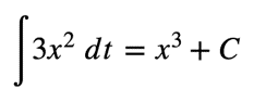
Integration Example
Consider the function, v(t) = x3. By
applying the power rule, we can easily find its derivative, v’(t)
= 3x2. The antiderivative of 3x2 is again x3
– we perform the reverse operation to obtain the original function.
Now suppose that we have a different function, g(t) = x3
+ 2. Its derivative is also 3x2, and so is the derivative of yet
another function, h(t) = x3 – 5. Both of these
functions (and other similar ones) have x3 as their
antiderivative. Hence, we specify the family of all antiderivatives of 3x2
by the indefinite integral:
The indefinite integral does not define the limits between which the area
under the curve is being calculated. The constant, C, is included to
compensate for the lack of information about the limits, or the starting point
of the sweep.
If we do have knowledge of the limits, then we can simply apply the second
fundamental theorem of calculus to compute the definite integral:

We can simply set C to
zero, because it will not change the result in this case.
No comments:
Post a Comment